This repository contains an organized DADA2 pipeline that you can clone and work directly on it.

It provides a directories structure so you can use it as the backbone of your project. You can find more info on structuring projects here.

Users need to have some bash and R knowledge along with understanding of the DADA2 algorithm.

Before starting, we highly recommend that you read at least one of the following tutorials:

• DADA2 pipeline official tutorial by benjjneb.
• DADA2 example workflow by astrobiomike.

The pipeline is divided into 4 big steps (plus an initial preprocessing step):

1. Statistics of reads, and cut adaptor.
2. Qscore profile plots.
3. Trimming reads and DADA2 algorithm.
4. Remove chimeras, merge runs and add taxonomy.
5. Check if output seqs contain duplicated reads (100% clustering).
   1. Extra: cluster, if necessary

To download the pipeline to your computer/cluster, open the terminal and go to your desired directory with cd. Then, type the following (assuming that you have git installed):

    git clone --depth 1 https://github.com/adriaaula/dada2_guidelines.git

(You can also download the repository from the Github server).

The directory dada2_guidelines/ will be copied to your computer. It contains the following files and subdirectories:

• README.md: this readme file.
• scripts/: where all scripts are located.
• data/:
  • logs/: all log files will be dumped here.
  • raw/: it contains a vanilla dataset, initially. It will contain your data. We recommend that instead of copying it, you use symlinks pointing to its original directory. You can easily create a symlink like this: ln -s /my/original/data/*fastq.gz data/raw/.
  • dada2/: where output files from DADA2 are written.

For everything to work properly, all scripts have to be submitted from the root directory of your project (dada_guidelines/ in this case). That is, the jobs have to be run (sent to the cluster) from the root directory, not from scripts/preprocessing. For each step, a bash script named XX_run is in the scripts/preprocessing. If you try to send them from scripts the program will be unable to find the desired files. This is the script with the SLURM header that has to be run. If you don't know anything about SLURM, our favorite bioinfo admin (@Pablo Sanchez) has a really nice tutorial in the marbits wiki.

You also can send this repository locally, but you will need to install all the programs used (cutadapt, seqkit, R, dada2 package, usearch and probably others :) ).

As explained in benjjneb's tutorial, DADA2 needs that your sequencing data meets the following criteria:

• Samples have been demultiplexed (one fastq file per sample).
• Non-biological nucleotides have been removed (e.g. primers, adapters).
• If paired-end sequencing data, the forward and reverse fastq files contain reads in matched order.

In this preprocessing step, we provide the script helper00_cutadapt.sh, which trims primers using cutadapt. The script outputs the trimmed R1 and R2 files plus a log file (in analysis/logs/cutadapt/) for each sample.

You will need the primers used in your study!

Finally, the following scripts are written assuming that your files have sample names written at the beggining of the filename and the pair information is written as R1/R2 (i.e. <sample-name>_R1.fastq). We recommend you to follow this naming or otherwise dig into the scripts and change the corresponding lines.

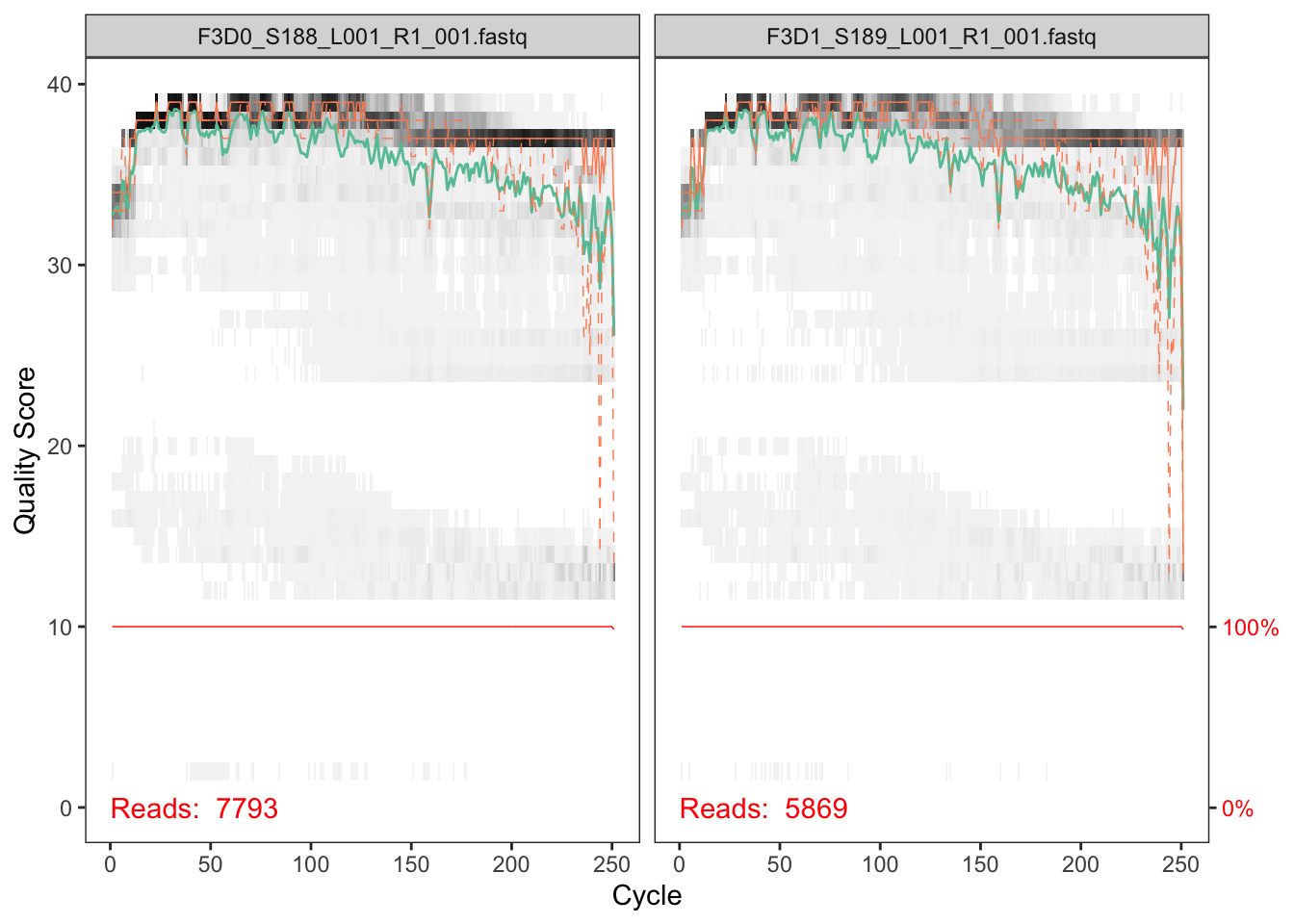
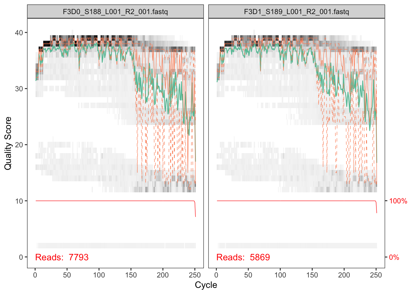
The first step in DADA2 is to check the quality of your sequencing data. To do so, we provide the script 0_run-qscore.sh, which calls the R script 0_qscore.R. Basically, it creates 2 pdf files (forward and reverse) with the q score profile of your first 9 samples (or all your samples if your dataset is smaller). The files generated look like this:

Inspecting the quality of your samples will help you to decide where to trim them in the following step. It is advisable to trim the most error-prone regions of your sequences (around 20 Qscore at least). But take into account that some error can be left, since the program is able to use it as valuable information for prediciting if a sequence is an error or a true biological variant. The trim length is based on how much your R1 and R2 are redundant. If your sequence is small, you can be quite conservative and cut widely. If your merging region is small, beware of cutting too much. Given the plots above, we should select the trimming length (around 240 for the forward read and 160 for the reverse one in this case).

To open pdfs both for the qscore plotting and the model from the next step, you will need to copy it to your local computer. The easiest way is to use scp. An example:

#Once you are in your local terminal
scp aauladell@marbits.csic.cmima.es:~/projects/dada2_guidelines/data/dada2/00_qprofiles/* ~/Downloads/.

Having decided where to trim (you'll most probably get it wrong the first time, this will be obvious by the amount of reads lost), we are able to jump to the next step, which is DADA2 itself. Here, the script 01_run-dada2.sh is provided, which calls the script 01_dada2-error-output.R. A value of max expected error (maxEE) for forward and reverse reads has to be provided along the trimming regions (truncLen). It is important to note that all reads not reaching the specified lengths will be discarded (so, if you are losing a lot of sequences, maybe you set too high the trimming value).

The main steps of this script are the following:

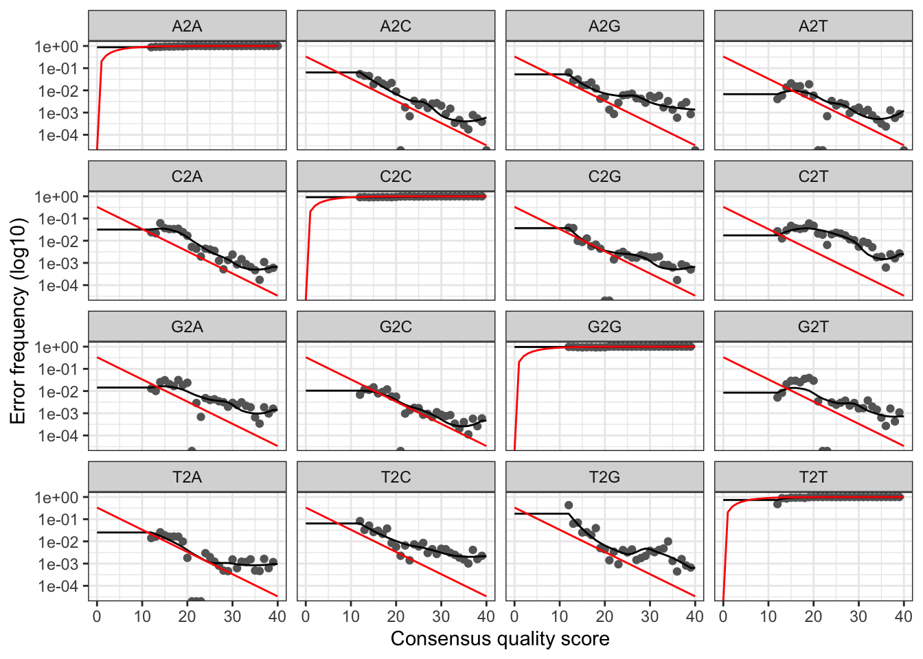
• Filter (maxEE) and trim (truncLen). Creates the data/filtered directory where it dumps the processed files.
• Learn errors. It creates a forward and reverse pdf files with the plotted error model of your samples. It is vital to check the results, since a bad error model will bring problems afterwards! A good error model example:

• Dereplication.
• Sample inference (dada).
• Merge paired reads.
• Build sequence table. Creates an ASV table (ASVs as rows, samples as columns)

The script also writes a file to track reads through the pipeline. If you see a big drop in reads in some step, maybe something went wrong.

In the same script, you can run multiple runs separately, which will be joined in the following step. Remeber that it is necessary to process each run individually since error distribution is different for each sequencing run.

In some cases, our dataset is splitted into multiple sequencing runs. Each of them should be processed separatedly with the dada2 algorithm, and here we will join the outputs (seqtab files) into a merged version with the abundance table, using the script 02_run_chimerarem_merge.sh. See the Big data for a detailed explanation.

Once the tables are merged, chimeric ASVs will be removed and we will obtain our final ASV counts table. The default method used to remove chimeras is 'consensus'. However, if you used pool=TRUE in the dada command you should use method 'pooled'. Now that you got rid of ugly chimeras, it's time to add taxonomy.

Here you can choose whether to use dada2 included classifier or DECIPHER. As far as we know, DECIPHER seems to retrieve better results (see paper for comparison) than the standard naive Bayesian classifier.

Anyway, we will use the script 03_run-add-taxonomy.sh, where you can specify the classification method you desire. Regardless of the method used, we recommend you to put your databases/training sets into data/assign_tax. If databases are already downloaded in your cluster, you can create a symlink (ln -s path/to/db data/assign_tax/) to your project.

Once you have your database ready, when using DECIPHER you have to decide at which confidence level you want to classify your ASVs. This is what people at DECIPHER say:

Select a minimum confidence threshold for classifications. We recommend using a confidence of 60% (very high) or 50% (high). Longer sequences are easier to classify because they contain more information, so a larger fraction of sequences will be classified at the same confidence threshold. The primary error mode of sequence classifiers is overclassification, where a sequence belonging to a novel group is assigned to an existing taxonomic group, and the overclassification rate is largely independent of sequence length. Therefore, it is not necessary to change the confidence threshold for shorter input sequences.

In the script we provide we set this level to 60, but feel free to play with it. After running your script, you will get a taxonomy table.

For dada2's classifier, you can specify the minimum bootstrap confidence for assigning a taxonomic level (minBoot). The default is 50.

We detected that, in some cases, merging tables from different runs gives reads that are identical but differ in length by a few base pairs. This has been included in the collapseNoMismatch function inside DADA2.

We provide here the script 04_run-ASV-clustering.sh, which creates a clustered seqtab at the desired percentage identity. Additionaly, it creates a table with ASVs to OTUs correspondence.

Some tips about the parameter selection!

• Cut your primers. cutadapt does the job really easy!

• If around 45-50 % of the reads are lost in the process of ASV generation, possibly some of the parameters have to be changed.

  • Are you sure that the primers from the FASTQ are removed?

• What maxee did you specify? If this is making many reads to be lost, you can specify a bigger maxee, and even different values for the F and R reads (for example c(2,4)). The algorithm will take into account the errors in the modelling phase, so this will not make your ASVs erroneus.

• Does the pair of reads overlap? By how many bases? It should be >= 20 nt.

If you follow the tutorial, at the end of the procedure a track analysis is generated specifying how many reads are lost along the whole procedure. It is the best way to know where it failed.

• In the trimming procedure, the truncLen cuts all the reads to an specific length and removes all reads being smaller. It is important then to know the average read length, since if you go too low with the trimming you will lose too much reads.

• In the pipeline of DADA2 there is a quality profile, you should be aware of it in deciding where to cut.

• For each run the trimming point is different, so if you are working on multiple runs each of them have to be processed separatedly and then joined together with mergeSequenceTables.

• You should have an analysis of the FASTQs. The av. length, the avg quality for each sample, and so on. Many of the problems with recovering most of the reads stem from having a low quality sample, or the reads not being properly amplified. seqkit is a good tool for this kind of information.

• The taxonomy assignation is done at the Species level only if only a 100%, exact matching. This can make that some Bacteria/Eukarya present differences in the identification at that level when comparing with OTU results. See a link explaining this in more detail here.

Adrià & Aleix
Backbone team 💀