<?xml version="1.0" encoding="utf-8"?><feed xmlns="http://www.w3.org/2005/Atom" ><generator uri="https://jekyllrb.com/" version="3.10.0">Jekyll</generator><link href="https://xgboost.ai/feed.xml" rel="self" type="application/atom+xml" /><link href="https://xgboost.ai/" rel="alternate" type="text/html" /><updated>2026-08-27T11:06:11+00:00</updated><id>https://xgboost.ai/feed.xml</id><title type="html">XGBoost</title><subtitle>Scalable and flexible gradient boosting</subtitle><author><name>XGBoost Contributors</name></author><entry><title type="html">Introducing the XGBoost Vector-Leaf Model</title><link href="https://xgboost.ai/2026/08/25/introducing-the-xgboost-vector-leaf-model" rel="alternate" type="text/html" title="Introducing the XGBoost Vector-Leaf Model" /><published>2026-08-25T00:00:00+00:00</published><updated>2026-08-25T00:00:00+00:00</updated><id>https://xgboost.ai/2026/08/25/introducing-the-xgboost-vector-leaf-model</id><content type="html" xml:base="https://xgboost.ai/2026/08/25/introducing-the-xgboost-vector-leaf-model"><![CDATA[<p>Most decision trees store a single number in each leaf. This works naturally for ordinary
regression, where a model predicts one value for every row. Many problems, however,
require several related predictions at once: multiclass classification, quantile and
expectile regression, and multi-output regression are common examples.</p>

<p>By default, XGBoost handles these problems by building one stack of scalar-leaf trees for
each output. The vector-leaf model offers another choice: build one shared tree whose
leaves hold a vector of predictions.</p>

<p>Across ten real-world multiclass datasets, vector leaves generally achieved lower held-out
loss and produced simpler models. When outputs benefit from using the same splits,
vector-leaf models can also train and predict faster and be less susceptible to spurious
features. In this post, we explore when shared tree structure helps and what trade-offs it
brings.</p>

<h2 id="getting-started">Getting started</h2>

<p>In XGBoost v3.4.1, the default <code class="language-plaintext highlighter-rouge">multi_strategy="one_output_per_tree"</code> builds a separate
scalar-leaf tree for each class at every boosting round. Set
<code class="language-plaintext highlighter-rouge">multi_strategy="multi_output_tree"</code> to build one shared tree with vector-valued leaves
instead.</p>

<p>The <code class="language-plaintext highlighter-rouge">hist</code> implementation supports CPU and CUDA training, categorical splits, and
reduced-gradient training. See the <a href="https://xgboost.readthedocs.io/en/stable/tutorials/multioutput.html">multi-output
tutorial</a> for details
and examples. Vector leaves were first prototyped for the CPU <code class="language-plaintext highlighter-rouge">hist</code> tree method in v2.0;
after several releases of refinement, v3.4.1 is the first feature-complete implementation
for <code class="language-plaintext highlighter-rouge">hist</code>.</p>

<p>This setting changes how the classes share model structure. Each vector leaf stores a
separate score update for every class, but all classes follow the same sequence of splits
that routes a row to that leaf. For a problem with 32 classes, one scalar boosting round
adds 32 trees, while one vector boosting round adds a single shared tree. This difference
can produce far fewer splits and a much simpler model.</p>

<p><img src="/images/blog/2026-08-25-introducing-the-xgboost-vector-leaf-model/scalar_vs_vector_leaf_trees.png" alt="Three scalar-leaf class trees compared with one shared vector-leaf tree" /></p>

<h2 id="why-share-a-tree">Why share a tree?</h2>

<p>Suppose a tree asks whether a pixel is dark, a playing card is an ace, or a sensor reading
exceeds a threshold. In a multiclass problem, the answer may be useful to several classes
at once. A vector-leaf tree asks the question once, then stores a different adjustment for
every class in the resulting leaf.</p>

<p>This is an appealing example of Occam’s razor: when one partition of the data works as
well as many separate partitions, prefer the simpler representation. It can be smaller and
faster to evaluate, and the shared structure can act as a useful modeling constraint,
making the model more likely to generalize well for unseen data.</p>

<p>The trade-off is that all outputs must use the same tree structure. This works best when
they benefit from similar features and split thresholds—a property we call <em>partition
compatibility</em>. In multiclass classification, for example, a question about whether a
region of an image contains ink may help distinguish several characters at once.</p>

<p>Partition compatibility is not the same as target correlation. Correlation says that
target values move together; it does not say that the targets need the same decision
boundaries. What matters here is whether the same split questions are useful across
outputs. If those questions and thresholds are largely unrelated, separate scalar trees
have more freedom.</p>

<h2 id="a-synthetic-example">A synthetic example</h2>

<p>To illustrate the benefit of compatible partitions, we generated a multi-output regression
problem with 32 normally distributed features. Every target combines those same set of
features with different weights and a small amount of random noise. The targets therefore
need different predictions, but they all benefit from the same basic split questions. We
generated <code class="language-plaintext highlighter-rouge">2^20</code> training rows and <code class="language-plaintext highlighter-rouge">2^18</code> test rows, then compared problems with 2, 4, 8,
16, and 32 outputs. Both strategies were trained for 128 boosting rounds. This
deliberately partition-compatible dataset is the favorable case for vector leaves.</p>

<p><img src="/images/blog/2026-08-25-introducing-the-xgboost-vector-leaf-model/computational_efficiency_gpu.png" alt="GPU scaling with compatible outputs. Error bars show variation across three timing repeats; the generated data are fixed." /></p>

<p>Both strategies retain essentially the same predictive error. Their complexity, however,
separates as the output count grows. At 32 outputs, the vector model is about one ninth of
the serialized size, and both training and prediction are faster. Separate scalar trees
largely repeat the same useful structure; the vector model represents it once.</p>

<h2 id="shared-partitions-resist-spurious-features">Shared partitions resist spurious features</h2>

<p>A second controlled experiment tests the regularizing effect of sharing a tree. We
generated a synthetic multiclass problem whose class probabilities come from one shared
tree over a small set of signal features. Each leaf holds class-specific logits, so the
true decision function is exactly partition-compatible.</p>

<p>We then added progressively larger sets of independent noise features. Within each paired
comparison, the rows, labels, and signal stay fixed, isolating the effect of giving the
models more irrelevant choices. We track how much the added noise worsens expected log
loss and, from the tree dumps, how much split gain the models assign to noise.</p>

<p><img src="/images/blog/2026-08-25-introducing-the-xgboost-vector-leaf-model/multiclass_noise_feature_selection.png" alt="Multiclass prediction error and gain assigned to noise features. Error bars show 95% confidence intervals over repeated paired datasets." /></p>

<p>The curves separate as more distractions become available. At the largest noise setting,
the scalar models devote more than twice as much split gain to irrelevant features and
suffer more than twice the increase in expected log loss. A scalar class tree can promote
a chance association found for one class, whereas a vector tree evaluates each split
jointly across all class-score dimensions. Class-specific fluctuations therefore have
less influence on the shared partition. Sharing does not eliminate noise splits, but it
makes them less competitive.</p>

<h2 id="what-happens-on-real-data">What happens on real data?</h2>

<p>We next compared the strategies on ten multiclass datasets ranging from 13,910 to more
than one million rows and from 6 to 1,000 classes. The applications include forest-cover
prediction, card hands, motor-drive diagnosis, gas sensing, character recognition, object
recognition, and Dionis, a large tabular benchmark with 355 classes from the ChaLearn
AutoML Challenge. The suite includes both balanced and heavily imbalanced class
distributions.</p>

<p>The figure shows the selected vector model relative to the selected scalar model, with
each model selected by validation loss before the test data were evaluated. The dashed
line is parity; points to the left favor vector leaves.  For example, a split ratio of
<code class="language-plaintext highlighter-rouge">0.25</code> means that the vector model uses one quarter as many splits as the scalar model.</p>

<p><img src="/images/blog/2026-08-25-introducing-the-xgboost-vector-leaf-model/vector_leaf_real_data_summary.png" alt="Vector/scalar ratios on ten multiclass datasets. Lower is better; dagger marks a round-cap hit." /></p>

<p>Vector leaves achieve lower held-out loss on nine of ten datasets and use fewer splits and
less disk space on all ten. Poker Hand is the standout, but the pattern also appears on
balanced datasets such as EMNIST and Devnagari, so class imbalance does not explain the
result by itself.</p>

<p>Some gains come with longer training. On Devnagari, the vector model uses about three
times as many boosting rounds to train. It nevertheless finishes substantially more
accurate and about one third the size. Letter Recognition improves both predictive quality
and training time, while Gas Sensor Drift retains a smaller advantage when trained on
earlier sensor batches and evaluated on later ones. Shared structure is an advantage when
it preserves enough predictive flexibility.</p>

<h2 id="a-practical-default-for-multiclass-classification">A practical default for multiclass classification</h2>

<p>These results make vector leaves a strong starting point for multiclass classification,
especially as the number of classes grows. Rather than treating <code class="language-plaintext highlighter-rouge">multi_output_tree</code> only
as a later optimization, it is reasonable to try it first and retain a scalar model as the
comparison.</p>

<p>Compared with scalar models, vector models may need more boosting rounds. Each scalar
round adds one tree per class, whereas each vector round adds only one shared tree. An
equal round limit therefore gives the scalar model much more tree structure. On K49 and
Devnagari, the vector models continued improving for substantially longer and eventually
became both more accurate and smaller than their scalar counterparts.</p>

<p>A lower learning rate is also worth pairing with the larger round cap. XGBoost’s default
learning rate is quite large. Reducing it makes each tree a smaller update and usually
enables more boosting rounds. The smaller steps can make the shared, multidimensional
updates easier to optimize. Dionis, for example, improved after its vector learning rate
was reduced. Early stopping can then select the useful number of rounds without committing
to the full cap.</p>

<h2 id="about-the-experiments">About the experiments</h2>

<p>Every real-data run used GPU histogram training and <code class="language-plaintext highlighter-rouge">QuantileDMatrix</code> with a DGX Spark.
Validation data controlled model selection and early stopping, and test data were
evaluated afterward. Random splits were stratified; Letter Recognition retained its
official test partition. Gas Sensor Drift used a time-ordered split because sensor
responses change over time. All these experiments use one deterministic split per dataset.</p>

<h2 id="summary">Summary</h2>

<p>Vector leaves replace one tree per output with one shared tree whose leaves hold
output-specific score updates. When outputs benefit from similar split questions, this can
improve predictive quality with far fewer splits and a much smaller model, while reducing
the influence of spurious features. The classification results make vector leaves a
compelling default to try.</p>

<p>For multiclass problems, start with a generous vector boosting rounds, include a lower
learning rate in the validation sweep, and let early stopping select the model. Keep the
result when it provides the right balance of predictive quality, model size, and training
cost for your application.</p>]]></content><author><name>Jiaming Yuan and Rory Mitchell</name></author><summary type="html"><![CDATA[Most decision trees store a single number in each leaf. This works naturally for ordinary regression, where a model predicts one value for every row. Many problems, however, require several related predictions at once: multiclass classification, quantile and expectile regression, and multi-output regression are common examples.]]></summary></entry><entry><title type="html">XGBoost 3.3.0 Release</title><link href="https://xgboost.ai/2026/07/21/xgboost-3-3-release" rel="alternate" type="text/html" title="XGBoost 3.3.0 Release" /><published>2026-07-21T00:00:00+00:00</published><updated>2026-07-21T00:00:00+00:00</updated><id>https://xgboost.ai/2026/07/21/xgboost-3-3-release</id><content type="html" xml:base="https://xgboost.ai/2026/07/21/xgboost-3-3-release"><![CDATA[<p>We are pleased to announce XGBoost 3.3.0. This release adds expectile regression,
enables categorical feature support by default, expands SHAP support for
vector-leaf multi-output trees, and includes a broad set of performance and
scalability improvements across CPU, GPU, distributed training, Python, JVM, and
the build system. In particular, GPU quantile sketching uses significantly less
memory for training.</p>

<p>XGBoost 3.3.0 is available from the usual package channels. The complete release
notes are available in the
<a href="https://xgboost.readthedocs.io/en/latest/changes/v3.3.0.html">XGBoost documentation</a>,
and release artifacts are available on
<a href="https://github.com/dmlc/xgboost/releases/tag/v3.3.0">GitHub</a>.</p>

<p>
  <img src="/images/blog/xgboost-3-3-larger-datasets.png" alt="Train even larger datasets with XGBoost 3.3" style="display: block; max-width: 480px; width: 100%; height: auto; margin: 0 auto;" />
</p>

<h2 id="faster-quantile-sketching-and-distributed-training">Faster quantile sketching and distributed training</h2>

<p>Quantile sketching received a substantial refactor in 3.3.0. The internals are
simpler, the weighted quantile sketch implementation is improved, and GPU
quantile sketching uses significantly less memory.</p>

<p>These changes matter because quantile construction is a central part of the
histogram-based training pipeline. Reducing memory use and simplifying the
implementation improves robustness for large datasets, wide datasets, and GPU
workloads where memory pressure often decides whether a job fits.</p>

<p>Distributed quantile construction is also more efficient in this release, using
tree reductions to improve scalability. XGBoost no longer requires all-to-all
collective connections for distributed training, and users can now customize the
worker port when deploying distributed jobs.</p>

<h2 id="expectile-regression">Expectile regression</h2>

<p>This release adds expectile regression, giving practitioners another tool for
risk-sensitive forecasting, uncertainty-aware modeling, and applications where
overprediction and underprediction carry different costs. It is available
through the new <code class="language-plaintext highlighter-rouge">reg:expectileerror</code> objective, the <code class="language-plaintext highlighter-rouge">expectile</code> metric, and the
<code class="language-plaintext highlighter-rouge">expectile_alpha</code> parameter.</p>

<p>Expectile regression is useful when users want an asymmetric squared-loss
analogue of quantile regression. It gives a smooth objective for estimating
different parts of the conditional response distribution, while retaining a
squared-error style penalty.</p>

<p>Multiple expectiles are supported, allowing users to train models for several
asymmetric targets in a single configuration. Unlike quantile regression,
expectile curves do not suffer from crossing, which makes them easier to use
when estimating multiple levels of the response distribution together. This
complements XGBoost’s existing regression objectives.</p>

<h2 id="categorical-features-are-on-by-default">Categorical features are on by default</h2>

<p>Categorical feature support is now enabled by default. Users no longer need to
set <code class="language-plaintext highlighter-rouge">enable_categorical=True</code> in the common case. The parameter remains available
for users who need to disable categorical handling explicitly.</p>

<p>This change reflects the maturity of categorical support in XGBoost and makes
the Python and dataframe workflows a little more natural. Dataframes with
categorical columns can be passed into XGBoost without an extra opt-in step,
making the default behavior match what many users already expect from modern
tabular machine learning libraries.</p>

<p>The CPU <code class="language-plaintext highlighter-rouge">hist</code> tree method also gained one-hot categorical split support for the
work-in-progress vector-leaf model. Vector-leaf trees are still under active
development, but this release continues to close gaps in the feature set.</p>

<h2 id="shap-support-for-vector-leaf-trees">SHAP support for vector-leaf trees</h2>

<p>XGBoost 3.3.0 expands SHAP support for vector-leaf multi-output trees. Exact SHAP
contribution and interaction prediction are now available for vector-leaf
multi-output trees on both CPU and GPU.</p>

<p>This is an important step for multi-output models. Vector-leaf trees can model
relationships across targets directly by storing a vector of weights in each
leaf, but users also need the same interpretability tools they rely on for
single-output models. With this release, multi-output workflows gain a more
complete explanation story.</p>

<p>The TreeSHAP implementation has also been updated for improved numerical
stability and faster execution with <code class="language-plaintext highlighter-rouge">QuadratureTreeSHAP</code> <a href="#references">[1]</a>.</p>

<h2 id="cpu-and-gpu-performance-improvements">CPU and GPU performance improvements</h2>

<p>On CPUs, histogram building has been optimized for wide datasets with column
block tiling. XGBoost can also detect CPU cache sizes through Linux sysfs on
aarch64, improving its ability to choose efficient execution strategies on
modern ARM platforms.</p>

<p>On GPUs, sampling now uses Philox for faster random number generation. This
release also continues the wider work on reducing GPU memory pressure and
improving the efficiency of the training pipeline.</p>

<p>Training with sampling is now more reproducible within a single session. XGBoost
uses a local random number generator and serializes the RNG state in the model
configuration, so pickled models can retain that state across save/load
boundaries. This helps when training multiple sampled models in the same process.</p>

<h2 id="python-and-spark-updates">Python and Spark updates</h2>

<p>The minimum supported Python version is now Python 3.12. This lets the project
remove older compatibility paths and focus testing on actively supported Python
versions.</p>

<p>The Python package also adds PySpark support for Spark Connect ML. This improves
compatibility with the newer Spark client-server workflow and keeps the XGBoost
Spark integration moving with the broader Spark ecosystem.</p>

<p>The release includes dataframe validation improvements as well. XGBoost now
requires <code class="language-plaintext highlighter-rouge">Enum</code> support from Polars and validates that pandas column names are
unique, helping users catch ambiguous feature inputs earlier.</p>

<p>Several Python fixes and cleanups are included: default verbose behavior is now
consistent between <code class="language-plaintext highlighter-rouge">XGBClassifier.fit</code> and <code class="language-plaintext highlighter-rouge">XGBRegressor.fit</code>, <code class="language-plaintext highlighter-rouge">python -OO</code>
crashes from missing docstrings have been fixed, boolean indicator features are
handled in <code class="language-plaintext highlighter-rouge">trees_to_dataframe</code>, and validation messages around feature
information and deprecated functions have been improved.</p>

<h2 id="jvm-build-and-platform-updates">JVM, build, and platform updates</h2>

<p>The JVM packages now document Spark 4.0 compatibility. Regressor and ranker
pipelines support columnar input, Java packages include automatic module names,
and <code class="language-plaintext highlighter-rouge">xgboost4j</code> supports FreeBSD.</p>

<p>On the build and platform side, XGBoost 3.3.0 adds support for Visual Studio
2026, updates CUDA Toolkit support, and fixes a number of CMake, macOS, and
packaging issues. Linux packaging now uses a versioned shared object.</p>

<h2 id="deprecation-notice">Deprecation notice</h2>

<p>The <code class="language-plaintext highlighter-rouge">gblinear</code> booster is deprecated in XGBoost 3.3.0 and will be removed in a
future release. The linear model feature in XGBoost has been a niche feature and
has not been as actively maintained as the tree algorithms. It also does not
support or align with many capabilities in modern XGBoost, such as categorical
splits, interaction constraints, monotone constraints, and TreeSHAP-style
explanations.</p>

<p>XGBoost is primarily a decision tree library, and we have decided to focus
development on the tree algorithms and on keeping the interface consistent for
the features users rely on most. Users relying on <code class="language-plaintext highlighter-rouge">gblinear</code> should start
planning migrations to other estimators or workflows.</p>

<h2 id="upgrade">Upgrade</h2>

<p>For Python users, upgrade with:</p>

<div class="language-sh highlighter-rouge"><div class="highlight"><pre class="highlight"><code>pip <span class="nb">install</span> <span class="nt">--upgrade</span> xgboost
</code></pre></div></div>

<p>For conda users:</p>

<div class="language-sh highlighter-rouge"><div class="highlight"><pre class="highlight"><code>conda <span class="nb">install</span> <span class="nt">-c</span> conda-forge xgboost
</code></pre></div></div>

<p>Please see the
<a href="https://xgboost.readthedocs.io/en/latest/install.html">installation guide</a> for
platform-specific instructions, and the
<a href="https://xgboost.readthedocs.io/en/latest/changes/v3.3.0.html">3.3.0 release notes</a>
for the full list of changes.</p>

<h2 id="references">References</h2>

<p>[1] Wettenstein R, Mitchell R, Yu P. (2026) Quadrature-TreeSHAP: Depth-Independent TreeSHAP and Shapley Interactions. <a href="https://arxiv.org/abs/2605.04497">arXiv:2605.04497</a>.</p>

<p>Many thanks to everyone who contributed code, reviews, testing, documentation,
bug reports, and release work for XGBoost 3.3.0.</p>]]></content><author><name>Jiaming Yuan and Rory Mitchell</name></author><summary type="html"><![CDATA[We are pleased to announce XGBoost 3.3.0. This release adds expectile regression, enables categorical feature support by default, expands SHAP support for vector-leaf multi-output trees, and includes a broad set of performance and scalability improvements across CPU, GPU, distributed training, Python, JVM, and the build system. In particular, GPU quantile sketching uses significantly less memory for training.]]></summary></entry><entry><title type="html">Updates to the XGBoost GPU algorithms</title><link href="https://xgboost.ai/2018/07/04/gpu-xgboost-update" rel="alternate" type="text/html" title="Updates to the XGBoost GPU algorithms" /><published>2018-07-04T00:00:00+00:00</published><updated>2018-07-04T00:00:00+00:00</updated><id>https://xgboost.ai/2018/07/04/gpu-xgboost-update</id><content type="html" xml:base="https://xgboost.ai/2018/07/04/gpu-xgboost-update"><![CDATA[<p>It has been one and a half years since <a href="https://xgboost.ai/2016/12/14/GPU-accelerated-xgboost.html">our last article</a> announcing the first ever GPU accelerated gradient boosting algorithm. GPU algorithms in XGBoost have been in continuous development over this time, adding new features, faster algorithms (much much faster), and improvements to usability. This blog post accompanies the paper <a href="http://arxiv.org/abs/1806.11248">XGBoost: Scalable GPU Accelerated Learning</a> <a href="#references">[1]</a> and describes some of these improvements.</p>

<h3 id="histogram-based-tree-construction-algorithms">Histogram based tree construction algorithms</h3>
<p>Decision tree construction algorithms typically work by recursively partitioning a set of training instances into smaller and smaller subsets in feature space. These partitions are found by searching over the training instances to find a decision rule that optimises for the training objective. While still effectively linear time these algorithms are slow because searching for the decision rule at the current level requires passing over every training instance. The algorithm can be made considerably faster through discretization of the input features.</p>

<p>Our primary decision tree construction algorithm is now a histogram based method such as that used in <a href="#references">[2]</a>,<a href="#references">[3]</a>. This means that we find quantiles over the input feature space and discretize our training examples into this space. Gradients from the training examples at each boosting iteration can then be summed into histogram ‘bins’ according to the now discrete features. Finding optimal splits for a decision tree then reduces to the simpler problem of searching over histogram bins in a discrete space.</p>

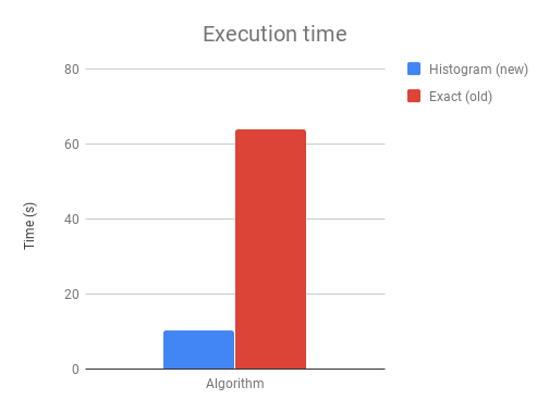
<p>The end result of this is a significantly faster and more memory efficient algorithm that still retains its accuracy.</p>

<p><img src="https://raw.githubusercontent.com/dmlc/web-data/master/xgboost/gpu/execution_time.png" alt="Execution time" /></p>

<p>The above chart shows the difference in execution time on a 1M*50 binary classification problem with 500 boosting iterations.</p>

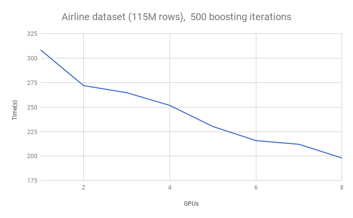
<h3 id="multi-gpu-support">Multi-GPU support</h3>
<p>Our histogram algorithm has full multi-GPU support using the NCCL library for scalable communication between GPUs. This means we can do things like run XGBoost on an AWS P3 instance with eight GPUs. The below chart shows the runtime on the 115M row airline dataset as we increase the number of GPUs:</p>

<p><img src="https://raw.githubusercontent.com/dmlc/web-data/master/xgboost/gpu/gpu_scalability.png" alt="Multi-GPU performance" /></p>

<p>Because of the efficient AllReduce communication primitives, communication throughput is constant as the number of GPUs is increased. Communication costs are also invariant to the number of training examples because only summary histogram statistics are shared. The data set is evenly distributed between GPUs. This allows us to scale up to datasets that cannot fit on a single GPU and use the full device memory capacity of multi-GPU systems.</p>

<h3 id="data-compression">Data compression</h3>

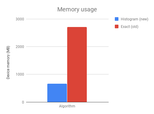
<p>Our current algorithm is also much more memory efficient than the original algorithm published in <a href="#references">[4]</a>. This is achieved largely through data compression of the input matrix after discretization. For example, if we use 256 histogram bins per feature and 50 features, there are only 256*50 unique feature values in the entire input matrix. By using bit compression we can store each matrix element using only log2(256*50)=14 bits per matrix element in a sparse CSR format. For comparison, a naive CSR storage format would typically cost a minimum of 64 bits per matrix element.</p>

<p><img src="https://raw.githubusercontent.com/dmlc/web-data/master/xgboost/gpu/memory_usage.png" alt="Memory usage" /></p>

<p>The above chart shows the device memory requirements for a 1M*50 binary classification problem on the histogram algorithm and the exact algorithm.</p>

<h3 id="gpu-prediction-and-gradient-calculation-algorithms">GPU prediction and gradient calculation algorithms</h3>
<p>Traditionally, tree construction algorithms account for most of the time spent in a gradient boosting algorithm. This changed after we developed significantly faster tree algorithms and other parts of the gradient boosting process began to create bottlenecks.</p>

<p>Prediction occurs every iteration in gradient boosting in order to calculate the gradients (residuals) for the next iteration. Users may also want to monitor performance on a test or validation set. This adds up to a large amount of computation on the CPU. We map this computation to a GPU kernel for a performance improvement of between 5-10x in prediction time. Note that this improvement is for memory that is already stored on the GPU. When used for an unseen dataset, prediction algorithms will be slower due to the time taken to copy the matrix to the GPU (i.e. these prediction algorithms are designed for training but not deployment of models).</p>

<p>We also introduce GPU accelerated objective function calculation for some tasks. These can be enabled by setting the objective function as one of:</p>
<div class="language-plaintext highlighter-rouge"><div class="highlight"><pre class="highlight"><code>"gpu:reg:linear", "gpu:reg:logistic", "gpu:binary:logistic", gpu:binary:logitraw"
</code></pre></div></div>

<p>Moving more parts of the gradient boosting pipeline onto the device removes computational bottlenecks as well as reducing the need to copy memory back and forth between the CPU and GPU across the limited bandwidth PCIe bus. Eventually we hope to move the entire pipeline to the device.</p>

<h2 id="benchmarking-against-other-gbm-algorithms">Benchmarking against other GBM algorithms</h2>

<p>Below are some benchmarks against other gradient boosting algorithms on an 8 GPU cloud computing instance. Instructions for reproducing these benchmarks <a href="https://github.com/RAMitchell/GBM-Benchmarks">can be found here</a>.</p>

<table>
  <thead>
    <tr>
      <th> </th>
      <th>YearPrediction</th>
      <th> </th>
      <th>Synthetic</th>
      <th> </th>
      <th>Higgs</th>
      <th> </th>
      <th>Cover Type</th>
      <th> </th>
      <th>Bosch</th>
      <th> </th>
      <th>Airline</th>
      <th> </th>
    </tr>
  </thead>
  <tbody>
    <tr>
      <td> </td>
      <td>Time(s)</td>
      <td>RMSE</td>
      <td>Time(s)</td>
      <td>RMSE</td>
      <td>Time(s)</td>
      <td>Accuracy</td>
      <td>Time(s)</td>
      <td>Accuracy</td>
      <td>Time(s)</td>
      <td>Accuracy</td>
      <td>Time(s)</td>
      <td>Accuracy</td>
    </tr>
    <tr>
      <td>xgb-cpu-hist</td>
      <td>216.71</td>
      <td>8.8794</td>
      <td>580.72</td>
      <td>13.6105</td>
      <td>509.29</td>
      <td>74.74</td>
      <td>3532.26</td>
      <td>89.2</td>
      <td>810.36</td>
      <td>99.45</td>
      <td>1948.26</td>
      <td>74.94</td>
    </tr>
    <tr>
      <td>xgb-gpu-hist</td>
      <td>30.39</td>
      <td>8.8799</td>
      <td>43.14</td>
      <td>13.4606</td>
      <td>38.41</td>
      <td>74.75</td>
      <td>107.70</td>
      <td>89.34</td>
      <td>27.97</td>
      <td>99.44</td>
      <td>110.29</td>
      <td>74.95</td>
    </tr>
    <tr>
      <td>lightgbm-cpu</td>
      <td>30.82</td>
      <td>8.8777</td>
      <td>463.79</td>
      <td>13.585</td>
      <td>330.25</td>
      <td>74.74</td>
      <td>186.27</td>
      <td>89.28</td>
      <td>162.29</td>
      <td>99.44</td>
      <td>916.04</td>
      <td>75.05</td>
    </tr>
    <tr>
      <td>lightgbm-gpu</td>
      <td>25.39</td>
      <td>8.8777</td>
      <td>576.67</td>
      <td>13.585</td>
      <td>725.91</td>
      <td>74.7</td>
      <td>383.03</td>
      <td>89.26</td>
      <td>409.93</td>
      <td>99.44</td>
      <td>614.74</td>
      <td>74.99</td>
    </tr>
    <tr>
      <td>cat-cpu</td>
      <td>39.93</td>
      <td>8.9933</td>
      <td>426.31</td>
      <td>9.387</td>
      <td>393.21</td>
      <td>74.06</td>
      <td>306.17</td>
      <td>85.14</td>
      <td>255.72</td>
      <td>99.44</td>
      <td>2949.04</td>
      <td>72.66</td>
    </tr>
    <tr>
      <td>cat-gpu</td>
      <td>10.15</td>
      <td>9.0637</td>
      <td>36.66</td>
      <td>9.3805</td>
      <td>30.37</td>
      <td>74.08</td>
      <td>N/A</td>
      <td>N/A</td>
      <td>N/A</td>
      <td>N/A</td>
      <td>303.36</td>
      <td>72.77</td>
    </tr>
  </tbody>
</table>

<h2 id="installation-and-usage">Installation and usage</h2>
<p>From XGBoost version 0.72 onwards, installation with GPU support for python on linux platforms is as simple as:</p>

<div class="language-sh highlighter-rouge"><div class="highlight"><pre class="highlight"><code>pip <span class="nb">install </span>xgboost
</code></pre></div></div>

<p>Users of other platforms will still need to <a href="https://xgboost.readthedocs.io/en/latest/build.html#building-with-gpu-support">build from source</a>, although prebuilt Windows packages are on the roadmap.</p>

<p>To use our new fast algorithms simply set the “tree_method” parameter to “gpu_hist” in your existing XGBoost script.</p>

<p>Simple examples using the XGBoost Python API and sklearn API:</p>

<div class="language-python highlighter-rouge"><div class="highlight"><pre class="highlight"><code><span class="kn">import</span> <span class="nn">xgboost</span> <span class="k">as</span> <span class="n">xgb</span>
<span class="kn">from</span> <span class="nn">sklearn.datasets</span> <span class="kn">import</span> <span class="n">load_boston</span>

<span class="n">boston</span> <span class="o">=</span> <span class="n">load_boston</span><span class="p">()</span>

<span class="c1"># XGBoost API example
</span><span class="n">params</span> <span class="o">=</span> <span class="p">{</span><span class="s">'tree_method'</span><span class="p">:</span> <span class="s">'gpu_hist'</span><span class="p">,</span> <span class="s">'max_depth'</span><span class="p">:</span> <span class="mi">3</span><span class="p">,</span> <span class="s">'learning_rate'</span><span class="p">:</span> <span class="mf">0.1</span><span class="p">}</span>
<span class="n">dtrain</span> <span class="o">=</span> <span class="n">xgb</span><span class="p">.</span><span class="n">DMatrix</span><span class="p">(</span><span class="n">boston</span><span class="p">.</span><span class="n">data</span><span class="p">,</span> <span class="n">boston</span><span class="p">.</span><span class="n">target</span><span class="p">)</span>
<span class="n">xgb</span><span class="p">.</span><span class="n">train</span><span class="p">(</span><span class="n">params</span><span class="p">,</span> <span class="n">dtrain</span><span class="p">,</span> <span class="n">evals</span><span class="o">=</span><span class="p">[(</span><span class="n">dtrain</span><span class="p">,</span> <span class="s">"train"</span><span class="p">)])</span>

<span class="c1"># sklearn API example
</span><span class="n">gbm</span> <span class="o">=</span> <span class="n">xgb</span><span class="p">.</span><span class="n">XGBRegressor</span><span class="p">(</span><span class="n">n_estimators</span><span class="o">=</span><span class="mi">10</span><span class="p">,</span> <span class="n">tree_method</span><span class="o">=</span><span class="s">'gpu_hist'</span><span class="p">)</span>
<span class="n">gbm</span><span class="p">.</span><span class="n">fit</span><span class="p">(</span><span class="n">boston</span><span class="p">.</span><span class="n">data</span><span class="p">,</span> <span class="n">boston</span><span class="p">.</span><span class="n">target</span><span class="p">,</span> <span class="n">eval_set</span><span class="o">=</span><span class="p">[(</span><span class="n">boston</span><span class="p">.</span><span class="n">data</span><span class="p">,</span> <span class="n">boston</span><span class="p">.</span><span class="n">target</span><span class="p">)])</span>
</code></pre></div></div>

<p>Output:</p>

<div class="language-sh highlighter-rouge"><div class="highlight"><pre class="highlight"><code><span class="o">[</span>01:12:20] Allocated 0MB on <span class="o">[</span>0] Tesla K80, 11352MB remaining.
<span class="o">[</span>01:12:20] Allocated 0MB on <span class="o">[</span>0] Tesla K80, 11351MB remaining.
<span class="o">[</span>01:12:20] Allocated 0MB on <span class="o">[</span>0] Tesla K80, 11350MB remaining.
<span class="o">[</span>0]     train-rmse:21.6024
<span class="o">[</span>1]     train-rmse:19.5554
<span class="o">[</span>2]     train-rmse:17.7153
<span class="o">[</span>3]     train-rmse:16.0624
<span class="o">[</span>4]     train-rmse:14.5719
<span class="o">[</span>5]     train-rmse:13.2413
<span class="o">[</span>6]     train-rmse:12.0342
<span class="o">[</span>7]     train-rmse:10.9578
<span class="o">[</span>8]     train-rmse:9.97791
<span class="o">[</span>9]     train-rmse:9.10676
<span class="o">[</span>01:12:20] Allocated 0MB on <span class="o">[</span>0] Tesla K80, 11352MB remaining.
<span class="o">[</span>01:12:20] Allocated 0MB on <span class="o">[</span>0] Tesla K80, 11351MB remaining.
<span class="o">[</span>01:12:20] Allocated 0MB on <span class="o">[</span>0] Tesla K80, 11350MB remaining.
<span class="o">[</span>0]     validation_0-rmse:21.6024
<span class="o">[</span>1]     validation_0-rmse:19.5554
<span class="o">[</span>2]     validation_0-rmse:17.7153
<span class="o">[</span>3]     validation_0-rmse:16.0624
<span class="o">[</span>4]     validation_0-rmse:14.5719
<span class="o">[</span>5]     validation_0-rmse:13.2413
<span class="o">[</span>6]     validation_0-rmse:12.0342
<span class="o">[</span>7]     validation_0-rmse:10.9578
<span class="o">[</span>8]     validation_0-rmse:9.97791
<span class="o">[</span>9]     validation_0-rmse:9.10676

</code></pre></div></div>

<h2 id="author">Author</h2>
<p>Rory Mitchell is a PhD student at the University of Waikato and works for H2O.ai.</p>

<p>Special thanks to all contributors of the XGBoost GPU project, in particular Andrey Adinets and Thejaswi Rao from Nvidia for significant algorithm improvements.</p>

<h2 id="references">References</h2>
<p>[1] Rory Mitchell, Andrey Adinets, Thejaswi Rao: “XGBoost: Scalable GPU Accelerated Learning”, 2018; http://arxiv.org/abs/1806.11248.</p>

<p>[2] Keck, Thomas. “FastBDT: A speed-optimized and cache-friendly implementation of stochastic gradient-boosted decision trees for multivariate classification.” arXiv preprint arXiv:1609.06119 (2016).</p>

<p>[3] Ke, Guolin, et al. “Lightgbm: A highly efficient gradient boosting decision tree.” Advances in Neural Information Processing Systems. 2017.</p>

<p>[4] Mitchell, Rory, and Eibe Frank. “Accelerating the XGBoost algorithm using GPU computing.” PeerJ Computer Science 3 (2017): e127.</p>]]></content><author><name>Rory Mitchell</name></author><summary type="html"><![CDATA[It has been one and a half years since our last article announcing the first ever GPU accelerated gradient boosting algorithm. GPU algorithms in XGBoost have been in continuous development over this time, adding new features, faster algorithms (much much faster), and improvements to usability. This blog post accompanies the paper XGBoost: Scalable GPU Accelerated Learning [1] and describes some of these improvements.]]></summary></entry><entry><title type="html">GPU Accelerated XGBoost</title><link href="https://xgboost.ai/2016/12/14/GPU-accelerated-xgboost" rel="alternate" type="text/html" title="GPU Accelerated XGBoost" /><published>2016-12-14T00:00:00+00:00</published><updated>2016-12-14T00:00:00+00:00</updated><id>https://xgboost.ai/2016/12/14/GPU-accelerated-xgboost</id><content type="html" xml:base="https://xgboost.ai/2016/12/14/GPU-accelerated-xgboost"><![CDATA[<p><strong><em>Update 2016/12/23:</em></strong>
Some of our benchmarks were incorrect due to a wrong compiler flag. These have all been updated below.</p>

<hr />

<p>Decision tree learning and gradient boosting have until recently been the domain of multicore CPUs. Here we showcase a new plugin providing GPU acceleration for the <a href="https://github.com/dmlc/xgboost">XGBoost library</a>. The plugin provides significant speedups over multicore CPUs for large datasets.</p>

<p>The plugin can be found at:
https://github.com/dmlc/xgboost/tree/master/plugin/updater_gpu</p>

<p>Before talking about the GPU plugin we briefly explain the XGBoost algorithm.</p>

<h2 id="xgboost-for-classification-and-regression">XGBoost for classification and regression</h2>
<p>XGBoost is a powerful tool for solving classification and regression problems in a supervised learning setting. It is an implementation of a generalised <a href="https://en.wikipedia.org/wiki/Gradient_boosting">gradient boosting</a> algorithm designed to offer high-performance, multicore scalability and distributed machine scalability.</p>

<p>The gradient boosting algorithm is an <a href="https://en.wikipedia.org/wiki/Ensemble_learning">ensemble learning</a> technique that builds many predictive models. Together these smaller models produce much stronger predictions than any single model alone. In particular for gradient boosting, we create these smaller models sequentially, where each new model directly addresses the weaknesses in the previous models.</p>

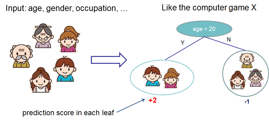
<p>While many types of models can be used in a boosting algorithm, in practice we almost always use <a href="https://en.wikipedia.org/wiki/Decision_tree_learning">decision trees</a>. Below we show an example of a decision tree that predicts if a person likes computer games based on their age, and gender. Given a new example to predict, we input the example at the root of the tree and follow the decision rules until reaching a leaf node with a prediction.</p>

<p><img src="https://raw.githubusercontent.com/dmlc/web-data/master/xgboost/model/cart.png" alt="" /></p>

<p>Given an ensemble of more than one tree we can combine the predictions to obtain a stronger prediction.
<img src="https://raw.githubusercontent.com/dmlc/web-data/master/xgboost/model/twocart.png" alt="" /></p>

<p>It is not uncommon to use XGBoost to create several thousand models such as the above, with each model incrementally improving the result from the previous models.</p>

<p>You may ask why should I care about gradient boosting when machine learning seems to be all about deep learning? The answer is that it works very well for structured data.</p>

<p>XGBoost has become so successful with the Kaggle data science community, to the point of <a href="https://www.import.io/post/how-to-win-a-kaggle-competition/">“winning practically every competition in the structured data category”</a>.</p>

<h2 id="gpu-acceleration">GPU Acceleration</h2>
<p>Machine learning tasks with XGBoost can take many hours to run. To achieve state-of-the-art prediction results we often want to create thousands of trees and test out many different parameter combinations. It would be nice if users could put their powerful and otherwise idle graphics cards to use accelerating this task.</p>

<p>GPUs launch many thousands of parallel threads at a time and can provide significant speedups for many compute intensive tasks that can be formulated as a parallel algorithm.</p>

<p>Luckily the decision tree construction algorithm may be formulated in parallel, allowing us to accelerate boosting iterations. Note that we parallelise the construction of individual trees - the boosting process itself has a serial dependency.</p>

<h2 id="how-fast-is-it">How fast is it?</h2>
<p>The following benchmarks show a performance comparison of GPUs against multicore CPUs for 500 boosting iterations. The new Pascal Titan X shows some nice performance improvements of up to 5.57x as compared to an i7 CPU. The Titan is also able to process the entire 10M row Higgs dataset in its 12GB of memory.</p>

<table>
  <thead>
    <tr>
      <th>Dataset</th>
      <th>Instances</th>
      <th>Features</th>
      <th>i7-6700K</th>
      <th>Titan X (pascal)</th>
      <th>Speedup</th>
    </tr>
  </thead>
  <tbody>
    <tr>
      <td>Yahoo LTR</td>
      <td>473,134</td>
      <td>700</td>
      <td>877</td>
      <td>277</td>
      <td>3.16</td>
    </tr>
    <tr>
      <td>Higgs</td>
      <td>10,500,000</td>
      <td>28</td>
      <td>14504</td>
      <td>3052</td>
      <td>4.75</td>
    </tr>
    <tr>
      <td>Bosch</td>
      <td>1,183,747</td>
      <td>968</td>
      <td>3294</td>
      <td>591</td>
      <td>5.57</td>
    </tr>
  </tbody>
</table>

<p>We also tested the Titan X against a server with 2x Xeon E5-2695v2 CPUs (24 cores in total) on the Yahoo learning to rank dataset. The GPU outperforms the CPUs by about 1.2x. This is a nice result considering the Titan X costs $1200 and the 2x Xeon CPUs cost almost $5000.</p>

<p><img src="https://github.com/dmlc/web-data/raw/master/xgboost/gpu/yahooltr_xeon_titan.png" alt="" /></p>

<h2 id="how-does-it-work">How does it work?</h2>
<p>The XGBoost algorithm requires scanning across gradient/hessian values and using these partial sums to evaluate the quality of splits at every possible split in the training set. The GPU XGBoost algorithm makes use of fast parallel prefix sum operations to scan through all possible splits as well as parallel radix sorting to repartition data. It builds a decision tree for a given boosting iteration one level at a time, processing the entire dataset concurrently on the GPU.</p>

<p>The algorithm also switches between two modes. The first mode processes node groups in interleaved order using specialised multiscan/multireduce operations. This provides better performance at lower levels in the tree  when there are fewer leaf nodes. At later levels we switched to using radix sort to repartition the data and perform more conventional scan/reduce operations.</p>

<h2 id="how-do-i-use-it">How do I use it?</h2>
<p>To use the GPU algorithm add the single parameter:</p>
<div class="language-python highlighter-rouge"><div class="highlight"><pre class="highlight"><code><span class="c1"># Python example
</span><span class="n">param</span><span class="p">[</span><span class="s">'updater'</span><span class="p">]</span> <span class="o">=</span> <span class="s">'grow_gpu'</span>
</code></pre></div></div>

<p>XGBoost must be built from source using the cmake build system, following the instructions <a href="https://github.com/dmlc/xgboost/tree/master/plugin/updater_gpu">here</a>.</p>

<p>The plug-in may be used through the Python or CLI interfaces at this time. <a href="https://github.com/dmlc/xgboost/tree/master/demo/gpu_acceleration">A demo is available</a> showing how to use the GPU algorithm to accelerate a cross validation task on a large dataset.</p>

<h2 id="about-the-author">About the author</h2>
<p>The XGBoost GPU plugin is contributed by <a href="https://github.com/RAMitchell">Rory Mitchell</a>. The project was a part of a Masters degree dissertation at Waikato University.</p>

<p>Many thanks to the XGBoost authors and contributors!</p>]]></content><author><name>Rory Mitchell</name></author><summary type="html"><![CDATA[Update 2016/12/23: Some of our benchmarks were incorrect due to a wrong compiler flag. These have all been updated below.]]></summary></entry><entry><title type="html">A Full Integration of XGBoost and Apache Spark</title><link href="https://xgboost.ai/2016/10/26/a-full-integration-of-xgboost-and-spark" rel="alternate" type="text/html" title="A Full Integration of XGBoost and Apache Spark" /><published>2016-10-26T08:00:00+00:00</published><updated>2016-10-26T08:00:00+00:00</updated><id>https://xgboost.ai/2016/10/26/a-full-integration-of-xgboost-and-spark</id><content type="html" xml:base="https://xgboost.ai/2016/10/26/a-full-integration-of-xgboost-and-spark"><![CDATA[<h2 id="introduction">Introduction</h2>

<p>On March 2016, we released the first version of <a href="http://dmlc.ml/2016/03/14/xgboost4j-portable-distributed-xgboost-in-spark-flink-and-dataflow.html">XGBoost4J</a>, which is a set of packages providing Java/Scala interfaces of XGBoost and the integration with prevalent JVM-based distributed data processing platforms, like Spark/Flink.</p>

<p>The integrations with Spark/Flink, a.k.a. <b>XGBoost4J-Spark</b> and <b>XGBoost-Flink</b>, receive the tremendous positive feedbacks from the community. It enables users to build a unified pipeline, embedding  XGBoost into the data processing system based on the widely-deployed frameworks like Spark. The following figure shows the general architecture of such a pipeline with the first version of <b>XGBoost4J-Spark</b>, where the data processing is based on the low-level <a href="http://spark.apache.org/docs/latest/programming-guide.html#resilient-distributed-datasets-rdds">Resilient Distributed Dataset (RDD)</a> abstraction.</p>

<p><img src="https://raw.githubusercontent.com/dmlc/web-data/master/xgboost/unified_pipeline.png" alt="XGBoost4J Architecture" /></p>

<p>In the last months, we have a lot of communication with the users and gain the deeper understanding of the users’ latest usage scenario and requirements:</p>

<ul>
  <li>
    <p>XGBoost keeps gaining more and more deployments in the production environment and the adoption in machine learning competitions <a href="http://datascience.la/xgboost-workshop-and-meetup-talk-with-tianqi-chen/">Link</a>.</p>
  </li>
  <li>
    <p>While Spark is still the mainstream data processing tool in most of scenarios, more and more users are porting their RDD-based Spark programs to <a href="http://spark.apache.org/docs/latest/sql-programming-guide.html">DataFrame/Dataset APIs</a> for the well-designed interfaces to manipulate structured data and the <a href="https://databricks.com/blog/2016/07/26/introducing-apache-spark-2-0.html">significant performance improvement</a>.</p>
  </li>
  <li>
    <p>Spark itself has presented a clear roadmap that DataFrame/Dataset would be the base of the latest and future features, e.g. latest version of <a href="http://spark.apache.org/docs/latest/ml-guide.html">ML pipeline</a> and <a href="http://spark.apache.org/docs/latest/structured-streaming-programming-guide.html">Structured Streaming</a>.</p>
  </li>
</ul>

<p>Based on these feedbacks from the users, we observe a gap between the original RDD-based XGBoost4J-Spark and the users’ latest usage scenario as well as the future direction of Spark ecosystem. To fill this gap, we start working on the <b><i>integration of XGBoost and Spark’s DataFrame/Dataset abstraction</i></b> in September. In this blog, we will introduce <b>the latest version of XGBoost4J-Spark</b> which allows the user to work with DataFrame/Dataset directly and embed XGBoost to Spark’s ML pipeline seamlessly.</p>

<h2 id="a-full-integration-of-xgboost-and-dataframedataset">A Full Integration of XGBoost and DataFrame/Dataset</h2>

<p>The following figure illustrates the new pipeline architecture with the latest XGBoost4J-Spark.</p>

<p><img src="https://raw.githubusercontent.com/dmlc/web-data/master/xgboost/unified_pipeline_new.png" alt="XGBoost4J New Architecture" /></p>

<p>Being different with the previous version, users are able to use both low- and high-level memory abstraction in Spark, i.e. RDD and DataFrame/Dataset. The DataFrame/Dataset abstraction grants the user to manipulate structured datasets and utilize the built-in routines in Spark or User Defined Functions (UDF) to explore the value distribution in columns before they feed data into the machine learning phase in the pipeline. In the following example, the structured sales records can be saved in a JSON file, parsed as DataFrame through Spark’s API and feed to train XGBoost model in two lines of Scala code.</p>

<div class="language-scala highlighter-rouge"><div class="highlight"><pre class="highlight"><code><span class="c1">// load sales records saved in json files</span>
<span class="k">val</span> <span class="nv">salesDF</span> <span class="k">=</span> <span class="nv">spark</span><span class="o">.</span><span class="py">read</span><span class="o">.</span><span class="py">json</span><span class="o">(</span><span class="s">"sales.json"</span><span class="o">)</span>
<span class="c1">// call XGBoost API to train with the DataFrame-represented training set</span>
<span class="k">val</span> <span class="nv">xgboostModel</span> <span class="k">=</span> <span class="nv">XGBoost</span><span class="o">.</span><span class="py">trainWithDataFrame</span><span class="o">(</span>
      <span class="n">salesDF</span><span class="o">,</span> <span class="n">paramMap</span><span class="o">,</span> <span class="n">numRound</span><span class="o">,</span> <span class="n">nWorkers</span><span class="o">,</span> <span class="n">useExternalMemory</span><span class="o">)</span>
</code></pre></div></div>

<p>By integrating with DataFrame/Dataset, XGBoost4J-Spark not only enables users to call DataFrame/Dataset APIs directly but also make  DataFrame/Dataset-based Spark features available to XGBoost users, e.g. ML Package.</p>

<h3 id="integration-with-ml-package">Integration with ML Package</h3>

<p>ML package of Spark provides a set of convenient tools for feature extraction/transformation/selection. Additionally, with the model selection tool in ML package, users can select the best model through an automatic parameter searching process which is defined with through ML package APIs. After integrating with DataFrame/Dataset abstraction, these charming features in ML package are also available to XGBoost users.</p>

<h4 id="feature-extractiontransformationselection">Feature Extraction/Transformation/Selection</h4>

<p>The following example shows a feature transformer which converts the string-typed storeType feature to the numeric storeTypeIndex. The transformed DataFrame is then fed to train XGBoost model.</p>

<div class="language-scala highlighter-rouge"><div class="highlight"><pre class="highlight"><code><span class="k">import</span> <span class="nn">org.apache.spark.ml.feature.StringIndexer</span>

<span class="c1">// load sales records saved in json files</span>
<span class="k">val</span> <span class="nv">salesDF</span> <span class="k">=</span> <span class="nv">spark</span><span class="o">.</span><span class="py">read</span><span class="o">.</span><span class="py">json</span><span class="o">(</span><span class="s">"sales.json"</span><span class="o">)</span>

<span class="c1">// transfrom the string-represented storeType feature to numeric storeTypeIndex</span>
<span class="k">val</span> <span class="nv">indexer</span> <span class="k">=</span> <span class="k">new</span> <span class="nc">StringIndexer</span><span class="o">()</span>
  <span class="o">.</span><span class="py">setInputCol</span><span class="o">(</span><span class="s">"storeType"</span><span class="o">)</span>
  <span class="o">.</span><span class="py">setOutputCol</span><span class="o">(</span><span class="s">"storeTypeIndex"</span><span class="o">)</span>
<span class="c1">// drop the extra column</span>
<span class="k">val</span> <span class="nv">indexed</span> <span class="k">=</span> <span class="nv">indexer</span><span class="o">.</span><span class="py">fit</span><span class="o">(</span><span class="n">salesDF</span><span class="o">).</span><span class="py">transform</span><span class="o">(</span><span class="n">df</span><span class="o">).</span><span class="py">drop</span><span class="o">(</span><span class="s">"storeType"</span><span class="o">)</span>

<span class="c1">// use the transformed dataframe as training dataset</span>
<span class="k">val</span> <span class="nv">xgboostModel</span> <span class="k">=</span> <span class="nv">XGBoost</span><span class="o">.</span><span class="py">trainWithDataFrame</span><span class="o">(</span>
      <span class="n">indexed</span><span class="o">,</span> <span class="n">paramMap</span><span class="o">,</span> <span class="n">numRound</span><span class="o">,</span> <span class="n">nWorkers</span><span class="o">,</span> <span class="n">useExternalMemory</span><span class="o">)</span>
</code></pre></div></div>

<h4 id="pipelining">Pipelining</h4>

<p>Spark ML package allows the user to build a complete pipeline from feature extraction/transformation/selection to model training. We integrate XGBoost with ML package and make it feasible to embed XGBoost into such a pipeline seamlessly. The following example shows how to build such a pipeline consisting of feature transformers and the XGBoost estimator.</p>

<div class="language-scala highlighter-rouge"><div class="highlight"><pre class="highlight"><code><span class="k">import</span> <span class="nn">org.apache.spark.ml.feature.StringIndexer</span>

<span class="c1">// load sales records saved in json files</span>
<span class="k">val</span> <span class="nv">salesDF</span> <span class="k">=</span> <span class="nv">spark</span><span class="o">.</span><span class="py">read</span><span class="o">.</span><span class="py">json</span><span class="o">(</span><span class="s">"sales.json"</span><span class="o">)</span>

<span class="c1">// transfrom the string-represented storeType feature to numeric storeTypeIndex</span>
<span class="k">val</span> <span class="nv">indexer</span> <span class="k">=</span> <span class="k">new</span> <span class="nc">StringIndexer</span><span class="o">()</span>
  <span class="o">.</span><span class="py">setInputCol</span><span class="o">(</span><span class="s">"storeType"</span><span class="o">)</span>
  <span class="o">.</span><span class="py">setOutputCol</span><span class="o">(</span><span class="s">"storeTypeIndex"</span><span class="o">)</span>

<span class="c1">// assemble the columns in dataframe into a vector</span>
<span class="k">val</span> <span class="nv">vectorAssembler</span> <span class="k">=</span> <span class="k">new</span> <span class="nc">VectorAssembler</span><span class="o">()</span>
      <span class="o">.</span><span class="py">setInputCols</span><span class="o">(</span><span class="nc">Array</span><span class="o">(</span><span class="s">"storeId"</span><span class="o">,</span> <span class="s">"storeTypeIndex"</span><span class="o">,</span> <span class="o">...))</span>
      <span class="o">.</span><span class="py">setOutputCol</span><span class="o">(</span><span class="s">"features"</span><span class="o">)</span>

<span class="c1">// construct the pipeline       </span>
<span class="k">val</span> <span class="nv">pipeline</span> <span class="k">=</span> <span class="k">new</span> <span class="nc">Pipeline</span><span class="o">().</span><span class="py">setStages</span><span class="o">(</span>
      <span class="nc">Array</span><span class="o">(</span><span class="n">storeTypeIndexer</span><span class="o">,</span> <span class="o">...,</span> <span class="n">vectorAssembler</span><span class="o">,</span> <span class="k">new</span> <span class="nc">XGBoostEstimator</span><span class="o">(</span><span class="nc">Map</span><span class="o">[</span><span class="kt">String</span>, <span class="kt">Any</span><span class="o">](</span><span class="s">"num_rounds"</span> <span class="o">-&gt;</span> <span class="mi">100</span><span class="o">)))</span>

<span class="c1">// use the transformed dataframe as training dataset</span>
<span class="k">val</span> <span class="nv">xgboostModel</span> <span class="k">=</span> <span class="nv">pipeline</span><span class="o">.</span><span class="py">fit</span><span class="o">(</span><span class="n">salesDF</span><span class="o">)</span>

<span class="c1">// predict with the trained model</span>
<span class="k">val</span> <span class="nv">salesTestDF</span> <span class="k">=</span> <span class="nv">spark</span><span class="o">.</span><span class="py">read</span><span class="o">.</span><span class="py">json</span><span class="o">(</span><span class="s">"sales_test.json"</span><span class="o">)</span>
<span class="k">val</span> <span class="nv">salesRecordsWithPred</span> <span class="k">=</span> <span class="nv">xgboostModel</span><span class="o">.</span><span class="py">transform</span><span class="o">(</span><span class="n">salesTestDF</span><span class="o">)</span>

</code></pre></div></div>

<h4 id="model-selection">Model Selection</h4>

<p>The most critical operation to maximize the power of XGBoost is to select the optimal parameters for the model. Tuning parameters manually is a tedious and labor-consuming process. With the latest version of XGBoost4J-Spark, we can utilize the Spark model selecting tool to automate this process. The following example shows the code snippet utilizing <a href="http://spark.apache.org/docs/latest/api/scala/index.html#org.apache.spark.ml.tuning.TrainValidationSplit">TrainValidationSplit</a> and <a href="http://spark.apache.org/docs/latest/api/scala/index.html#org.apache.spark.ml.evaluation.RegressionEvaluator">RegressionEvaluator</a> to search the optimal combination of two XGBoost parameters, [max_depth and eta] (https://github.com/dmlc/xgboost/blob/master/doc/parameter.md). The model producing the minimum cost function value defined by RegressionEvaluator is selected and used to generate the prediction for the test set.</p>

<div class="language-scala highlighter-rouge"><div class="highlight"><pre class="highlight"><code><span class="c1">// create XGBoostEstimator </span>
<span class="k">val</span> <span class="nv">xgbEstimator</span> <span class="k">=</span> <span class="k">new</span> <span class="nc">XGBoostEstimator</span><span class="o">(</span><span class="n">xgboostParam</span><span class="o">).</span><span class="py">setFeaturesCol</span><span class="o">(</span><span class="s">"features"</span><span class="o">).</span>
      <span class="nf">setLabelCol</span><span class="o">(</span><span class="s">"sales"</span><span class="o">)</span>
<span class="k">val</span> <span class="nv">paramGrid</span> <span class="k">=</span> <span class="k">new</span> <span class="nc">ParamGridBuilder</span><span class="o">()</span>
      <span class="o">.</span><span class="py">addGrid</span><span class="o">(</span><span class="nv">xgbEstimator</span><span class="o">.</span><span class="py">maxDepth</span><span class="o">,</span> <span class="nc">Array</span><span class="o">(</span><span class="mi">5</span><span class="o">,</span> <span class="mi">6</span><span class="o">))</span>
      <span class="o">.</span><span class="py">addGrid</span><span class="o">(</span><span class="nv">xgbEstimator</span><span class="o">.</span><span class="py">eta</span><span class="o">,</span> <span class="nc">Array</span><span class="o">(</span><span class="mf">0.1</span><span class="o">,</span> <span class="mf">0.4</span><span class="o">))</span>
      <span class="o">.</span><span class="py">build</span><span class="o">()</span>
<span class="k">val</span> <span class="nv">tv</span> <span class="k">=</span> <span class="k">new</span> <span class="nc">TrainValidationSplit</span><span class="o">()</span>
      <span class="o">.</span><span class="py">setEstimator</span><span class="o">(</span><span class="n">xgbEstimator</span><span class="o">)</span>
      <span class="o">.</span><span class="py">setEvaluator</span><span class="o">(</span><span class="k">new</span> <span class="nc">RegressionEvaluator</span><span class="o">().</span><span class="py">setLabelCol</span><span class="o">(</span><span class="s">"sales"</span><span class="o">))</span>
      <span class="o">.</span><span class="py">setEstimatorParamMaps</span><span class="o">(</span><span class="n">paramGrid</span><span class="o">)</span>
      <span class="o">.</span><span class="py">setTrainRatio</span><span class="o">(</span><span class="mf">0.8</span><span class="o">)</span>  
<span class="k">val</span> <span class="nv">salesTestDF</span> <span class="k">=</span> <span class="nv">spark</span><span class="o">.</span><span class="py">read</span><span class="o">.</span><span class="py">json</span><span class="o">(</span><span class="s">"sales_test.json"</span><span class="o">)</span>
<span class="k">val</span> <span class="nv">salesRecordsWithPred</span> <span class="k">=</span> <span class="nv">xgboostModel</span><span class="o">.</span><span class="py">transform</span><span class="o">(</span><span class="n">salesTestDF</span><span class="o">)</span>
</code></pre></div></div>

<h2 id="summary">Summary</h2>

<p>Through the latest XGBoost4J-Spark, XGBoost users can build a more efficient data processing pipeline which works with DataFrame/Dataset APIs to handle the structured data with the excellent performance, and simultaneously embrace the powerful XGBoost to explore the insights from the dataset and transform this insight into action. Additionally, XGBoost4J-Spark seamlessly connect XGBoost with Spark ML package which makes the job of feature extraction/transformation/selection and parameter model much easier than before.</p>

<p>The latest version of XGBoost4J-Spark has been available in the [GitHub Repository] (https://github.com/dmlc/xgboost), and the latest API docs are in <a href="http://xgboost.readthedocs.io/en/latest/jvm/index.html">here</a>.</p>

<h2 id="portable-machine-learning-systems">Portable Machine Learning Systems</h2>

<p>XGBoost is one of the projects incubated by <a href="http://dmlc.ml/">Distributed Machine Learning Community (DMLC)</a>, which also creates several other popular projects on machine learning systems (<a href="https://github.com/dmlc/">Link</a>), e.g. one of the most popular deep learning frameworks, <a href="http://mxnet.io/">MXNet</a>. We strongly believe that machine learning solution should not be restricted to certain language or certain platform. We realize this design philosophy in several projects, like XGBoost and MXNet. We are willing to see more contributions from the community in this direction.</p>

<h2 id="further-readings">Further Readings</h2>

<p>If you are interested in knowing more about XGBoost, you can find rich resources in</p>

<ul>
  <li><a href="https://github.com/dmlc/xgboost">The github repository of XGBoost</a></li>
  <li><a href="http://xgboost.readthedocs.org/en/latest/index.html">The comprehensive documentation site for XGBoostl</a></li>
  <li><a href="http://xgboost.readthedocs.org/en/latest/model.html">An introduction to the gradient boosting model</a></li>
  <li><a href="xgboost.readthedocs.org/en/latest/R-package/index.html">Tutorials for the R package</a></li>
  <li><a href="http://xgboost.readthedocs.org/en/latest/parameter.html">Introduction of the Parameters</a></li>
  <li><a href="https://github.com/dmlc/xgboost/tree/master/demo">Awesome XGBoost, a curated list of examples, tutorials, blogs about XGBoost usecases</a></li>
</ul>]]></content><author><name>Nan Zhu</name></author><summary type="html"><![CDATA[Introduction]]></summary></entry><entry><title type="html">XGBoost4J: Portable Distributed XGBoost in Spark, Flink and Dataflow</title><link href="https://xgboost.ai/2016/03/14/xgboost4j-portable-distributed-xgboost-in-spark-flink-and-dataflow" rel="alternate" type="text/html" title="XGBoost4J: Portable Distributed XGBoost in Spark, Flink and Dataflow" /><published>2016-03-14T12:00:00+00:00</published><updated>2016-03-14T12:00:00+00:00</updated><id>https://xgboost.ai/2016/03/14/xgboost4j-portable-distributed-xgboost-in-spark-flink-and-dataflow</id><content type="html" xml:base="https://xgboost.ai/2016/03/14/xgboost4j-portable-distributed-xgboost-in-spark-flink-and-dataflow"><![CDATA[<h2 id="introduction">Introduction</h2>
<p><a href="https://github.com/dmlc/xgboost">XGBoost</a> is a library designed and optimized for tree boosting. Gradient boosting trees model is originally proposed by Friedman et al. By embracing multi-threads and introducing regularization, XGBoost delivers higher computational power and more accurate prediction.  <strong>More than half of the winning solutions in machine learning challenges</strong> hosted at Kaggle adopt XGBoost (<a href="https://github.com/dmlc/xgboost/tree/master/demo#machine-learning-challenge-winning-solutions">Incomplete list</a>).
XGBoost has provided native interfaces for  C++, R, python, Julia and Java users.
It is used by both <a href="https://github.com/dmlc/xgboost/tree/master/demo#usecases">data exploration and production scenarios</a> to solve real world machine learning problems.</p>

<p>The distributed XGBoost is described in the <a href="http://arxiv.org/abs/1603.02754">recently published paper</a>.
In short, the XGBoost system runs magnitudes faster than existing alternatives of distributed ML,
and uses far fewer resources. The reader is more than welcomed to refer to the paper for more details.</p>

<p>Despite the current great success, one of our ultimate goals is to make XGBoost even more available for all production scenario.
Programming languages and data processing/storage systems based on Java Virtual Machine (JVM) play the significant roles in the BigData ecosystem. <a href="http://hadoop.apache.org/">Hadoop</a>, <a href="http://spark.apache.org/">Spark</a> and more recently introduced <a href="http://flink.apache.org/">Flink</a> are very useful solutions to general large-scale data processing.</p>

<p>On the other side, the emerging demands of machine learning and deep learning
inspires many excellent machine learning libraries.
Many of these machine learning libraries(e.g. <a href="https://github.com/dmlc/xgboost">XGBoost</a>/<a href="https://github.com/dmlc/mxnet">MxNet</a>)
requires new computation abstraction and native support (e.g. C++ for GPU computing).
They are also often <a href="http://arxiv.org/abs/1603.02754">much more efficient</a>.</p>

<p>The gap between the implementation fundamentals of the general data processing frameworks and the more specific machine learning libraries/systems prohibits the smooth connection between these two types of systems, thus brings unnecessary inconvenience to the end user. The common workflow to the user is to utilize the systems like Spark/Flink to preprocess/clean data, pass the results to machine learning systems like <a href="https://github.com/dmlc/xgboost">XGBoost</a>/<a href="https://github.com/dmlc/mxnet">MxNet</a>)  via the file systems and then conduct the following machine learning phase. This process jumping across two types of systems creates certain inconvenience for the users and brings additional overhead to the operators of the infrastructure.</p>

<p>We want best of both worlds, so we can use the data processing frameworks like Spark and Flink toghether with
the best distributed machine learning solutions.
To resolve the situation, we introduce the new-brewed <a href="https://github.com/dmlc/xgboost/tree/master/jvm-packages">XGBoost4J</a>,
<b>XGBoost</b> for <b>J</b>VM Platform. We aim to provide the clean Java/Scala APIs and the integration with the most popular data processing systems developed in JVM-based languages.</p>

<h2 id="unix-philosophy-in-machine-learning">Unix Philosophy in Machine Learning</h2>

<p>XGBoost and XGBoost4J adopts Unix Philosophy.
XGBoost <strong>does its best in one thing – tree boosting</strong> and is <strong>being designed to work with other systems</strong>.
We strongly believe that machine learning solution should not be restricted to certain language or certain platform.</p>

<p>Specifically, users will be able to use distributed XGBoost in both Spark and Flink, and possibly more frameworks in Future.
We have made the API in a portable way so it <strong>can be easily ported to other Dataflow frameworks provided by the Cloud</strong>.
XGBoost4J shares its core with other XGBoost libraries, which means data scientists can use R/python
read and visualize the model trained distributedly.
It also means that user can start with single machine version for exploration,
which already can handle hundreds of million examples.</p>

<h2 id="system-overview">System Overview</h2>

<p>In the following Figure, we describe the overall architecture of XGBoost4J. XGBoost4J provides the Java/Scala API calling the core functionality of XGBoost library. Most importantly, it not only supports the single-machine model training, but also provides an abstraction layer which masks the difference of the underlying data processing engines and scales training to the distributed servers.</p>

<p><img src="https://raw.githubusercontent.com/dmlc/web-data/master/xgboost/xgboost4j.png" alt="XGBoost4J Architecture" /></p>

<p>By calling the XGBoost4J API, users can scale the model training to the cluster. XGBoost4J calls the running instance of XGBoost worker in Spark/Flink task and run them across the cluster. The communication among the distributed model training tasks and the XGBoost4J runtime environment go through [Rabit] (https://github.com/dmlc/rabit).</p>

<p>With the abstraction of XGBoost4J, users can build an unified data analytic application ranging from Extract-Transform-Loading, data exploration, machine learning model training and the final data product service. The following figure illustrate an example application built on top of Apache Spark. The application seamlessly embeds XGBoost into the processing pipeline and exchange data with other Spark-based processing phase through Spark’s distributed memory layer.</p>

<p><img src="https://raw.githubusercontent.com/dmlc/web-data/master/xgboost/unified_pipeline.png" alt="XGBoost4J Architecture" /></p>

<h2 id="single-machine-training-walk-through">Single-machine Training Walk-through</h2>

<p>In this section, we will work through the APIs of XGBoost4J by examples.
We will be using scala for demonstration, but we also have a complete API for java users.</p>

<p>To start the model training and evaluation, we need to prepare the training and test set:</p>

<div class="language-scala highlighter-rouge"><div class="highlight"><pre class="highlight"><code><span class="k">val</span> <span class="nv">trainMax</span> <span class="k">=</span> <span class="k">new</span> <span class="nc">DMatrix</span><span class="o">(</span><span class="s">"../../demo/data/agaricus.txt.train"</span><span class="o">)</span>
<span class="k">val</span> <span class="nv">testMax</span> <span class="k">=</span> <span class="k">new</span> <span class="nc">DMatrix</span><span class="o">(</span><span class="s">"../../demo/data/agaricus.txt.test"</span><span class="o">)</span>
</code></pre></div></div>

<p>After preparing the data, we can train our model:</p>

<div class="language-scala highlighter-rouge"><div class="highlight"><pre class="highlight"><code><span class="k">val</span> <span class="nv">params</span> <span class="k">=</span> <span class="k">new</span> <span class="nv">mutable</span><span class="o">.</span><span class="py">HashMap</span><span class="o">[</span><span class="kt">String</span>, <span class="kt">Any</span><span class="o">]()</span>
<span class="n">params</span> <span class="o">+=</span> <span class="s">"eta"</span> <span class="o">-&gt;</span> <span class="mf">1.0</span>
<span class="n">params</span> <span class="o">+=</span> <span class="s">"max_depth"</span> <span class="o">-&gt;</span> <span class="mi">2</span>
<span class="n">params</span> <span class="o">+=</span> <span class="s">"objective"</span> <span class="o">-&gt;</span> <span class="s">"binary:logistic"</span>

<span class="k">val</span> <span class="nv">watches</span> <span class="k">=</span> <span class="k">new</span> <span class="nv">mutable</span><span class="o">.</span><span class="py">HashMap</span><span class="o">[</span><span class="kt">String</span>, <span class="kt">DMatrix</span><span class="o">]</span>
<span class="n">watches</span> <span class="o">+=</span> <span class="s">"train"</span> <span class="o">-&gt;</span> <span class="n">trainMax</span>
<span class="n">watches</span> <span class="o">+=</span> <span class="s">"test"</span> <span class="o">-&gt;</span> <span class="n">testMax</span>

<span class="k">val</span> <span class="nv">round</span> <span class="k">=</span> <span class="mi">2</span>
<span class="c1">// train a model</span>
<span class="k">val</span> <span class="nv">booster</span> <span class="k">=</span> <span class="nv">XGBoost</span><span class="o">.</span><span class="py">train</span><span class="o">(</span><span class="n">trainMax</span><span class="o">,</span> <span class="nv">params</span><span class="o">.</span><span class="py">toMap</span><span class="o">,</span> <span class="n">round</span><span class="o">,</span> <span class="nv">watches</span><span class="o">.</span><span class="py">toMap</span><span class="o">)</span>
</code></pre></div></div>

<p>We then evaluate our model:</p>

<div class="language-scala highlighter-rouge"><div class="highlight"><pre class="highlight"><code><span class="k">val</span> <span class="nv">predicts</span> <span class="k">=</span> <span class="nv">booster</span><span class="o">.</span><span class="py">predict</span><span class="o">(</span><span class="n">testMax</span><span class="o">)</span>
</code></pre></div></div>

<p><code class="language-plaintext highlighter-rouge">predict</code> can output the predict results and you can define a customized evaluation method to derive your own metrics (see the example in (<a href="https://github.com/dmlc/xgboost/blob/master/jvm-packages/xgboost4j-example/src/main/java/ml/dmlc/xgboost4j/java/example/CustomObjective.java">Customized Evaluation Metric in Java</a>, [Customized Evaluation Metric in Scala] (https://github.com/dmlc/xgboost/blob/master/jvm-packages/xgboost4j-example/src/main/scala/ml/dmlc/xgboost4j/scala/example/CustomObjective.scala)).</p>

<h2 id="distributed-model-training-with-distributed-dataflow-frameworks">Distributed Model Training with Distributed Dataflow Frameworks</h2>

<p>The most exciting part in this XGBoost4J release is the integration with the Distributed Dataflow Framework. The most popular data processing frameworks fall into this category, e.g. <a href="http://spark.apache.org/">Apache Spark</a>, [Apache Flink] (http://flink.apache.org/), etc. In this part, we will walk through the steps to build the unified data analytic applications containing data preprocessing and distributed model training with Spark and Flink. (currently, we only provide Scala API for the integration with Spark and Flink)</p>

<p>Similar to the single-machine training, we need to prepare the training and test dataset.</p>

<h3 id="spark-example">Spark Example</h3>

<p>In Spark, the dataset is represented as the <a href="http://spark.apache.org/docs/latest/programming-guide.html#resilient-distributed-datasets-rdds">Resilient Distributed Dataset (RDD)</a>, we can utilize the Spark-distributed tools to parse libSVM file and wrap it as the RDD:</p>

<div class="language-scala highlighter-rouge"><div class="highlight"><pre class="highlight"><code><span class="k">val</span> <span class="nv">trainRDD</span> <span class="k">=</span> <span class="nv">MLUtils</span><span class="o">.</span><span class="py">loadLibSVMFile</span><span class="o">(</span><span class="n">sc</span><span class="o">,</span> <span class="n">inputTrainPath</span><span class="o">).</span><span class="py">repartition</span><span class="o">(</span><span class="nf">args</span><span class="o">(</span><span class="mi">1</span><span class="o">).</span><span class="py">toInt</span><span class="o">)</span>
</code></pre></div></div>

<p>We move forward to train the models:</p>

<div class="language-scala highlighter-rouge"><div class="highlight"><pre class="highlight"><code><span class="k">val</span> <span class="nv">xgboostModel</span> <span class="k">=</span> <span class="nv">XGBoost</span><span class="o">.</span><span class="py">train</span><span class="o">(</span><span class="n">trainRDD</span><span class="o">,</span> <span class="n">paramMap</span><span class="o">,</span> <span class="n">numRound</span><span class="o">,</span> <span class="n">numWorkers</span><span class="o">)</span>
</code></pre></div></div>

<p>The next step is to evaluate the model, you can either predict in local side or in a distributed fashion</p>

<div class="language-scala highlighter-rouge"><div class="highlight"><pre class="highlight"><code><span class="c1">// testSet is an RDD containing testset data represented as</span>
<span class="c1">// org.apache.spark.mllib.regression.LabeledPoint</span>
<span class="k">val</span> <span class="nv">testSet</span> <span class="k">=</span> <span class="nv">MLUtils</span><span class="o">.</span><span class="py">loadLibSVMFile</span><span class="o">(</span><span class="n">sc</span><span class="o">,</span> <span class="n">inputTestPath</span><span class="o">)</span>

<span class="c1">// local prediction</span>
<span class="c1">// import methods in DataUtils to convert Iterator[org.apache.spark.mllib.regression.LabeledPoint]</span>
<span class="c1">// to Iterator[ml.dmlc.xgboost4j.LabeledPoint] in automatic</span>
<span class="k">import</span> <span class="nn">DataUtils._</span>
<span class="nv">xgboostModel</span><span class="o">.</span><span class="py">predict</span><span class="o">(</span><span class="k">new</span> <span class="nc">DMatrix</span><span class="o">(</span><span class="nv">testSet</span><span class="o">.</span><span class="py">collect</span><span class="o">().</span><span class="py">iterator</span><span class="o">)</span>

<span class="c1">// distributed prediction</span>
<span class="nv">xgboostModel</span><span class="o">.</span><span class="py">predict</span><span class="o">(</span><span class="n">testSet</span><span class="o">)</span>
</code></pre></div></div>
<h3 id="flink-example">Flink example</h3>

<p>In Flink, we represent training data as Flink’s <a href="https://ci.apache.org/projects/flink/flink-docs-master/apis/batch/index.html">DataSet</a></p>

<div class="language-scala highlighter-rouge"><div class="highlight"><pre class="highlight"><code><span class="k">val</span> <span class="nv">trainData</span> <span class="k">=</span> <span class="nv">MLUtils</span><span class="o">.</span><span class="py">readLibSVM</span><span class="o">(</span><span class="n">env</span><span class="o">,</span> <span class="s">"/path/to/data/agaricus.txt.train"</span><span class="o">)</span>
</code></pre></div></div>

<p>Model Training can be done as follows</p>

<div class="language-scala highlighter-rouge"><div class="highlight"><pre class="highlight"><code><span class="k">val</span> <span class="nv">xgboostModel</span> <span class="k">=</span> <span class="nv">XGBoost</span><span class="o">.</span><span class="py">train</span><span class="o">(</span><span class="n">trainData</span><span class="o">,</span> <span class="n">paramMap</span><span class="o">,</span> <span class="n">round</span><span class="o">)</span>
</code></pre></div></div>

<p>Training and prediction.</p>

<div class="language-scala highlighter-rouge"><div class="highlight"><pre class="highlight"><code><span class="c1">// testData is a Dataset containing testset data represented as</span>
<span class="c1">// org.apache.flink.ml.math.Vector.LabeledVector</span>
<span class="k">val</span> <span class="nv">testData</span> <span class="k">=</span> <span class="nv">MLUtils</span><span class="o">.</span><span class="py">readLibSVM</span><span class="o">(</span><span class="n">env</span><span class="o">,</span> <span class="s">"/path/to/data/agaricus.txt.test"</span><span class="o">)</span>

<span class="c1">// local prediction</span>
<span class="nv">xgboostModel</span><span class="o">.</span><span class="py">predict</span><span class="o">(</span><span class="nv">testData</span><span class="o">.</span><span class="py">collect</span><span class="o">().</span><span class="py">iterator</span><span class="o">)</span>

<span class="c1">// distributed prediction</span>
<span class="nv">xgboostModel</span><span class="o">.</span><span class="py">predict</span><span class="o">(</span><span class="nv">testData</span><span class="o">.</span><span class="py">map</span><span class="o">{</span><span class="n">x</span> <span class="k">=&gt;</span> <span class="nv">x</span><span class="o">.</span><span class="py">vector</span><span class="o">})</span>
</code></pre></div></div>

<h2 id="road-map">Road Map</h2>

<p>It is the first release of XGBoost4J package, we are actively move forward for more charming features in the next release. You can watch our progress in <a href="https://github.com/dmlc/xgboost/issues/935">XGBoost4J Road Map</a>.</p>

<p>While we are trying our best to keep the minimum changes to the APIs, it is still subject to the incompatible changes.</p>

<h2 id="further-readings">Further Readings</h2>

<p>If you are interested in knowing more about XGBoost, you can find rich resources in</p>

<ul>
  <li><a href="https://github.com/dmlc/xgboost">The github repository of XGBoost</a></li>
  <li><a href="http://xgboost.readthedocs.org/en/latest/index.html">The comprehensive documentation site for XGBoostl</a></li>
  <li><a href="http://xgboost.readthedocs.org/en/latest/model.html">An introduction to the gradient boosting model</a></li>
  <li><a href="xgboost.readthedocs.org/en/latest/R-package/index.html">Tutorials for the R package</a></li>
  <li><a href="http://xgboost.readthedocs.org/en/latest/parameter.html">Introduction of the Parameters</a></li>
  <li><a href="https://github.com/dmlc/xgboost/tree/master/demo">Awesome XGBoost, a curated list of examples, tutorials, blogs about XGBoost usecases</a></li>
</ul>

<h2 id="acknowledgements">Acknowledgements</h2>

<p>We would like to send many thanks to <a href="https://github.com/yanqingmen">Zixuan Huang</a>, the early developer of XGBoost for Java (XGBoost for Java).</p>]]></content><author><name>Nan Zhu, Tianqi Chen</name></author><summary type="html"><![CDATA[Introduction XGBoost is a library designed and optimized for tree boosting. Gradient boosting trees model is originally proposed by Friedman et al. By embracing multi-threads and introducing regularization, XGBoost delivers higher computational power and more accurate prediction. More than half of the winning solutions in machine learning challenges hosted at Kaggle adopt XGBoost (Incomplete list). XGBoost has provided native interfaces for C++, R, python, Julia and Java users. It is used by both data exploration and production scenarios to solve real world machine learning problems.]]></summary></entry><entry><title type="html">An Introduction to XGBoost R package</title><link href="https://xgboost.ai/rstats/2016/03/10/xgboost" rel="alternate" type="text/html" title="An Introduction to XGBoost R package" /><published>2016-03-10T15:05:00+00:00</published><updated>2016-03-10T15:05:00+00:00</updated><id>https://xgboost.ai/rstats/2016/03/10/xgboost</id><content type="html" xml:base="https://xgboost.ai/rstats/2016/03/10/xgboost"><![CDATA[<h2 id="introduction">Introduction</h2>

<p><a href="https://github.com/dmlc/xgboost">XGBoost</a> is a library designed and optimized for boosting trees algorithms. Gradient boosting trees model is originally proposed by Friedman et al. The underlying algorithm of XGBoost is similar, specifically it is an extension of the classic gbm algorithm. By employing multi-threads and imposing regularization, XGBoost is able to utilize more computational power and get more accurate prediction. Please refer to <a href="http://xgboost.readthedocs.org/en/latest/model.html">this tutorial</a> for the details of the model.</p>

<p>One evidence of its accuracy is that XGBoost is used in more than half of the winning solutions in machine learning challenges hosted at <a href="https://www.kaggle.com/">Kaggle</a>. We have prepared <a href="https://github.com/dmlc/xgboost/tree/master/demo#machine-learning-challenge-winning-solutions">a (incomplete) list</a> of winning solutions.</p>

<p>There’re various high-level interfaces. Currently there are interfaces of XGBoost in C++, R, python, Julia, Java and Scala. The core functions in XGBoost are implemented in C++, thus it is easy to share models among different interfaces. This post is going to focus on the R package <code class="language-plaintext highlighter-rouge">xgboost</code>, which has a friendly user interface and comprehensive documentation. Based on the statistics from the <a href="http://cranlogs.r-pkg.org/badges/xgboost">RStudio CRAN mirror</a>, The package has been downloaded for more than 4,000 times in the last month.</p>

<p>The R package <code class="language-plaintext highlighter-rouge">xgboost</code> has won the 2016 John M. Chambers Statistical Software Award. From the very beginning of the work, our goal is to make a package which brings convenience and joy to the users. Thus we will introduce several details of the R pacakge <code class="language-plaintext highlighter-rouge">xgboost</code> that (we think) users would love to know.</p>

<h2 id="a-1-minute-beginners-guide">A 1-minute Beginner’s Guide</h2>

<p><code class="language-plaintext highlighter-rouge">xgboost</code> is available on both <a href="https://cran.r-project.org/web/packages/xgboost/index.html">CRAN</a> and <a href="https://github.com/dmlc/xgboost/tree/master/R-package">Github</a>. To install the stable/pre-compiled version from CRAN, simply run:</p>

<div class="language-r highlighter-rouge"><div class="highlight"><pre class="highlight"><code><span class="n">install.packages</span><span class="p">(</span><span class="s1">'xgboost'</span><span class="p">)</span><span class="w">
</span></code></pre></div></div>

<p>You can also install from our weekly updated drat repo:</p>

<div class="language-r highlighter-rouge"><div class="highlight"><pre class="highlight"><code><span class="n">install.packages</span><span class="p">(</span><span class="s2">"drat"</span><span class="p">,</span><span class="w"> </span><span class="n">repos</span><span class="o">=</span><span class="s2">"https://cran.rstudio.com"</span><span class="p">)</span><span class="w">
</span><span class="n">drat</span><span class="o">:::</span><span class="n">addRepo</span><span class="p">(</span><span class="s2">"dmlc"</span><span class="p">)</span><span class="w">
</span><span class="n">install.packages</span><span class="p">(</span><span class="s2">"xgboost"</span><span class="p">,</span><span class="w"> </span><span class="n">repos</span><span class="o">=</span><span class="s2">"http://dmlc.ml/drat/"</span><span class="p">,</span><span class="w"> </span><span class="n">type</span><span class="o">=</span><span class="s2">"source"</span><span class="p">)</span><span class="w">
</span></code></pre></div></div>

<p>In order to run a machine learning algorithm, we need a data set first. <code class="language-plaintext highlighter-rouge">xgboost</code> has a demo data set about mushrooms. This data set records biological attributes of different mushroom species, and the target is to predict whether it is poisonous. Users can load the data with</p>

<div class="language-r highlighter-rouge"><div class="highlight"><pre class="highlight"><code><span class="n">require</span><span class="p">(</span><span class="n">xgboost</span><span class="p">)</span><span class="w">

</span><span class="n">data</span><span class="p">(</span><span class="n">agaricus.train</span><span class="p">,</span><span class="w"> </span><span class="n">package</span><span class="o">=</span><span class="s1">'xgboost'</span><span class="p">)</span><span class="w">
</span><span class="n">data</span><span class="p">(</span><span class="n">agaricus.test</span><span class="p">,</span><span class="w"> </span><span class="n">package</span><span class="o">=</span><span class="s1">'xgboost'</span><span class="p">)</span><span class="w">
</span><span class="n">train</span><span class="w"> </span><span class="o">&lt;-</span><span class="w"> </span><span class="n">agaricus.train</span><span class="w">
</span><span class="n">test</span><span class="w"> </span><span class="o">&lt;-</span><span class="w"> </span><span class="n">agaricus.test</span><span class="w">
</span></code></pre></div></div>

<p>Each variable is a <code class="language-plaintext highlighter-rouge">list</code> containing two things, <code class="language-plaintext highlighter-rouge">label</code> and <code class="language-plaintext highlighter-rouge">data</code>. The next step is to feed this data to <code class="language-plaintext highlighter-rouge">xgboost</code>. Besides the data, we need to train the model with some other parameters:</p>

<ul>
  <li><code class="language-plaintext highlighter-rouge">nrounds</code>: the number of decision trees in the final model</li>
  <li><code class="language-plaintext highlighter-rouge">objective</code>: the training objective to use, where “binary:logistic” means a binary classifier.</li>
</ul>

<p>The simplest training command is as follows:</p>

<div class="language-r highlighter-rouge"><div class="highlight"><pre class="highlight"><code><span class="n">model</span><span class="w"> </span><span class="o">&lt;-</span><span class="w"> </span><span class="n">xgboost</span><span class="p">(</span><span class="n">data</span><span class="w"> </span><span class="o">=</span><span class="w"> </span><span class="n">train</span><span class="o">$</span><span class="n">data</span><span class="p">,</span><span class="w"> </span><span class="n">label</span><span class="w"> </span><span class="o">=</span><span class="w"> </span><span class="n">train</span><span class="o">$</span><span class="n">label</span><span class="p">,</span><span class="w">
                 </span><span class="n">nrounds</span><span class="w"> </span><span class="o">=</span><span class="w"> </span><span class="m">2</span><span class="p">,</span><span class="w"> </span><span class="n">objective</span><span class="w"> </span><span class="o">=</span><span class="w"> </span><span class="s2">"binary:logistic"</span><span class="p">)</span><span class="w">
</span></code></pre></div></div>

<div class="language-plaintext highlighter-rouge"><div class="highlight"><pre class="highlight"><code>## [0]	train-error:0.000614
## [1]	train-error:0.001228
</code></pre></div></div>

<p>We can make prediction on the test data set easily:</p>

<div class="language-r highlighter-rouge"><div class="highlight"><pre class="highlight"><code><span class="n">preds</span><span class="w"> </span><span class="o">=</span><span class="w"> </span><span class="n">predict</span><span class="p">(</span><span class="n">model</span><span class="p">,</span><span class="w"> </span><span class="n">test</span><span class="o">$</span><span class="n">data</span><span class="p">)</span><span class="w">
</span></code></pre></div></div>

<p>Sometimes it is important to use cross-validation to exam our model. In <code class="language-plaintext highlighter-rouge">xgboost</code> we provide a function <code class="language-plaintext highlighter-rouge">xgb.cv</code> to do that. Basically users can just copy every thing from <code class="language-plaintext highlighter-rouge">xgboost</code>, and specify <code class="language-plaintext highlighter-rouge">nfold</code>:</p>

<div class="language-r highlighter-rouge"><div class="highlight"><pre class="highlight"><code><span class="n">cv.res</span><span class="w"> </span><span class="o">&lt;-</span><span class="w"> </span><span class="n">xgb.cv</span><span class="p">(</span><span class="n">data</span><span class="w"> </span><span class="o">=</span><span class="w"> </span><span class="n">train</span><span class="o">$</span><span class="n">data</span><span class="p">,</span><span class="w"> </span><span class="n">label</span><span class="w"> </span><span class="o">=</span><span class="w"> </span><span class="n">train</span><span class="o">$</span><span class="n">label</span><span class="p">,</span><span class="w"> </span><span class="n">nfold</span><span class="w"> </span><span class="o">=</span><span class="w"> </span><span class="m">5</span><span class="p">,</span><span class="w">
                 </span><span class="n">nrounds</span><span class="w"> </span><span class="o">=</span><span class="w"> </span><span class="m">2</span><span class="p">,</span><span class="w"> </span><span class="n">objective</span><span class="w"> </span><span class="o">=</span><span class="w"> </span><span class="s2">"binary:logistic"</span><span class="p">)</span><span class="w">
</span></code></pre></div></div>

<div class="language-plaintext highlighter-rouge"><div class="highlight"><pre class="highlight"><code>## [0]	train-error:0.000921+0.000343	test-error:0.001228+0.000687
## [1]	train-error:0.001075+0.000172	test-error:0.001228+0.000687
</code></pre></div></div>

<p>To get to know more details about the usage of <code class="language-plaintext highlighter-rouge">xgboost</code>, please visit <a href="http://xgboost.readthedocs.org/en/latest/R-package/xgboostPresentation.html">our tutorial</a> for more information.</p>

<h2 id="efficient-algorithm">Efficient Algorithm</h2>

<p>If you have experiences in training models on a large data set, then you probably agree that waiting for the training to be done is boring. Time is a resource, so the training speed of an learning algorithm is important. This is determined by both algorithm and implementation. We pay attention to these issues when building <code class="language-plaintext highlighter-rouge">xgboost</code>, thus we are confident that <code class="language-plaintext highlighter-rouge">xgboost</code> is one of the fastest learning algorithm of gradient boosting algorithm. The reasons for the good efficiency are:</p>

<ul>
  <li>The computational part is implemented in C++.</li>
  <li>It can be multi-threaded on a single machine.</li>
  <li>It preprocesses the data before the training algorithm.</li>
</ul>

<p><img src="https://raw.githubusercontent.com/dmlc/web-data/master/xgboost/SpeedFigure.png" width="450px" /></p>

<p>This figure is generated with the dataset from <a href="https://www.kaggle.com/c/higgs-boson">the Higgs Boson Competition</a>. It can be described from two aspects:</p>

<ul>
  <li>With only one thread, the effect of preprocessing and C++ is already obvious.</li>
  <li>The multi-threading is almost linear with the number of threads, thus boosting the efficiency further.</li>
</ul>

<h2 id="convenient-interface">Convenient Interface</h2>

<p>As the developers of <code class="language-plaintext highlighter-rouge">xgboost</code>, we are also heavy users of <code class="language-plaintext highlighter-rouge">xgboost</code>. We value the experience on this tool. During the development, we try to shape the package to be user-friendly. Here are several details we would like to share, please click the title to visit the sample code.</p>

<p><strong><em>Customized Objective</em></strong></p>

<p><code class="language-plaintext highlighter-rouge">xgboost</code> can take customized objective. This means the model could be trained to optimize the objective defined by user. This is not often seen in other tools, since most of the algorithms are binded with a specific objective. With <code class="language-plaintext highlighter-rouge">xgboost</code>, one can train a model which maximize the work on the correct direction.</p>

<p>Let’s use log-likelihood as an demo. We define the following function to calculate the first and second order of gradient of the loss function:</p>

<div class="language-r highlighter-rouge"><div class="highlight"><pre class="highlight"><code><span class="n">loglossobj</span><span class="w"> </span><span class="o">&lt;-</span><span class="w"> </span><span class="k">function</span><span class="p">(</span><span class="n">preds</span><span class="p">,</span><span class="w"> </span><span class="n">dtrain</span><span class="p">)</span><span class="w"> </span><span class="p">{</span><span class="w">
  </span><span class="c1"># dtrain is the internal format of the training data</span><span class="w">
  </span><span class="c1"># We extract the labels from the training data</span><span class="w">
  </span><span class="n">labels</span><span class="w"> </span><span class="o">&lt;-</span><span class="w"> </span><span class="n">getinfo</span><span class="p">(</span><span class="n">dtrain</span><span class="p">,</span><span class="w"> </span><span class="s2">"label"</span><span class="p">)</span><span class="w">
  </span><span class="c1"># We compute the 1st and 2nd gradient, as grad and hess</span><span class="w">
  </span><span class="n">preds</span><span class="w"> </span><span class="o">&lt;-</span><span class="w"> </span><span class="m">1</span><span class="o">/</span><span class="p">(</span><span class="m">1</span><span class="w"> </span><span class="o">+</span><span class="w"> </span><span class="nf">exp</span><span class="p">(</span><span class="o">-</span><span class="n">preds</span><span class="p">))</span><span class="w">
  </span><span class="n">grad</span><span class="w"> </span><span class="o">&lt;-</span><span class="w"> </span><span class="n">preds</span><span class="w"> </span><span class="o">-</span><span class="w"> </span><span class="n">labels</span><span class="w">
  </span><span class="n">hess</span><span class="w"> </span><span class="o">&lt;-</span><span class="w"> </span><span class="n">preds</span><span class="w"> </span><span class="o">*</span><span class="w"> </span><span class="p">(</span><span class="m">1</span><span class="w"> </span><span class="o">-</span><span class="w"> </span><span class="n">preds</span><span class="p">)</span><span class="w">
  </span><span class="c1"># Return the result as a list</span><span class="w">
  </span><span class="nf">return</span><span class="p">(</span><span class="nf">list</span><span class="p">(</span><span class="n">grad</span><span class="w"> </span><span class="o">=</span><span class="w"> </span><span class="n">grad</span><span class="p">,</span><span class="w"> </span><span class="n">hess</span><span class="w"> </span><span class="o">=</span><span class="w"> </span><span class="n">hess</span><span class="p">))</span><span class="w">
</span><span class="p">}</span><span class="w">
</span></code></pre></div></div>

<p>Then we train the model as</p>

<div class="language-r highlighter-rouge"><div class="highlight"><pre class="highlight"><code><span class="n">model</span><span class="w"> </span><span class="o">&lt;-</span><span class="w"> </span><span class="n">xgboost</span><span class="p">(</span><span class="n">data</span><span class="w"> </span><span class="o">=</span><span class="w"> </span><span class="n">train</span><span class="o">$</span><span class="n">data</span><span class="p">,</span><span class="w"> </span><span class="n">label</span><span class="w"> </span><span class="o">=</span><span class="w"> </span><span class="n">train</span><span class="o">$</span><span class="n">label</span><span class="p">,</span><span class="w">
                 </span><span class="n">nrounds</span><span class="w"> </span><span class="o">=</span><span class="w"> </span><span class="m">2</span><span class="p">,</span><span class="w"> </span><span class="n">objective</span><span class="w"> </span><span class="o">=</span><span class="w"> </span><span class="n">loglossobj</span><span class="p">,</span><span class="w"> </span><span class="n">eval_metric</span><span class="w"> </span><span class="o">=</span><span class="w"> </span><span class="s2">"error"</span><span class="p">)</span><span class="w">
</span></code></pre></div></div>

<div class="language-plaintext highlighter-rouge"><div class="highlight"><pre class="highlight"><code>## [0]	train-error:0.001228
## [1]	train-error:0.001228
</code></pre></div></div>

<p>The result should be equivalent to <code class="language-plaintext highlighter-rouge">objective = "binary:logistic"</code>.</p>

<p><strong><em>Early Stopping</em></strong></p>

<p>A usual scenario is when we are not sure how many trees we need, we will firstly try some numbers and check the result. If the number we try is too small, we need to make it larger; If the number is too large, we are wasting time to wait for the termination. By setting the parameter <code class="language-plaintext highlighter-rouge">early_stopping</code>, <code class="language-plaintext highlighter-rouge">xgboost</code> will terminate the training process if the performance is getting worse in the iteration.</p>

<div class="language-r highlighter-rouge"><div class="highlight"><pre class="highlight"><code><span class="n">bst</span><span class="w"> </span><span class="o">&lt;-</span><span class="w"> </span><span class="n">xgb.cv</span><span class="p">(</span><span class="n">data</span><span class="w"> </span><span class="o">=</span><span class="w"> </span><span class="n">train</span><span class="o">$</span><span class="n">data</span><span class="p">,</span><span class="w"> </span><span class="n">label</span><span class="w"> </span><span class="o">=</span><span class="w"> </span><span class="n">train</span><span class="o">$</span><span class="n">label</span><span class="p">,</span><span class="w"> </span><span class="n">nfold</span><span class="w"> </span><span class="o">=</span><span class="w"> </span><span class="m">5</span><span class="p">,</span><span class="w">
              </span><span class="n">nrounds</span><span class="w"> </span><span class="o">=</span><span class="w"> </span><span class="m">20</span><span class="p">,</span><span class="w"> </span><span class="n">objective</span><span class="w"> </span><span class="o">=</span><span class="w"> </span><span class="s2">"binary:logistic"</span><span class="p">,</span><span class="w">
              </span><span class="n">early.stop.round</span><span class="w"> </span><span class="o">=</span><span class="w"> </span><span class="m">3</span><span class="p">,</span><span class="w"> </span><span class="n">maximize</span><span class="w"> </span><span class="o">=</span><span class="w"> </span><span class="kc">FALSE</span><span class="p">)</span><span class="w">
</span></code></pre></div></div>

<div class="language-plaintext highlighter-rouge"><div class="highlight"><pre class="highlight"><code>## [0]	train-error:0.000921+0.000343	test-error:0.001228+0.000686
## [1]	train-error:0.001228+0.000172	test-error:0.001228+0.000686
## [2]	train-error:0.000653+0.000442	test-error:0.001075+0.000875
## [3]	train-error:0.000422+0.000416	test-error:0.000767+0.000940
## [4]	train-error:0.000192+0.000429	test-error:0.000460+0.001029
## [5]	train-error:0.000192+0.000429	test-error:0.000460+0.001029
## [6]	train-error:0.000000+0.000000	test-error:0.000000+0.000000
## [7]	train-error:0.000000+0.000000	test-error:0.000000+0.000000
## [8]	train-error:0.000000+0.000000	test-error:0.000000+0.000000
## [9]	train-error:0.000000+0.000000	test-error:0.000000+0.000000
## Stopping. Best iteration: 7
</code></pre></div></div>

<p>Here we are doing cross validation. <code class="language-plaintext highlighter-rouge">early.stop.round = 3</code> means if the performance is not getting better for 3 steps, then the program will stop. <code class="language-plaintext highlighter-rouge">maximize = FALSE</code> means our goal is not to maximize the evaluation, where the default evaluation metric for binary classification is the classification error rate. We can see that even we ask the model to train 20 trees, it stopped after the performance is perfect.</p>

<p><strong><em>Continue Training</em></strong></p>

<p>Sometimes we might want to try to do 1000 iterations and check the result, then decide if we need another 1000 ones. Usually the second step could only be done by starting from the beginning, again. In <code class="language-plaintext highlighter-rouge">xgboost</code> users can continue the training on the previous model, thus the second step will cost you the time for the additional iterations only. The theoratical reason that we are capable to do this is because each tree is only trained based the prediction result of the previous trees. Once we get the prediction by the current trees, we can start to train the next one.</p>

<p>This feature involves with the internal data format of <code class="language-plaintext highlighter-rouge">xgboost</code>: <code class="language-plaintext highlighter-rouge">xgb.DMatrix</code>. An <code class="language-plaintext highlighter-rouge">xgb.DMatrix</code> object contains the features, target and other side informations, e.g. weights, missing values.</p>

<p>First, let us define an <code class="language-plaintext highlighter-rouge">xgb.DMatrix</code> object for this data:</p>

<div class="language-r highlighter-rouge"><div class="highlight"><pre class="highlight"><code><span class="n">dtrain</span><span class="w"> </span><span class="o">&lt;-</span><span class="w"> </span><span class="n">xgb.DMatrix</span><span class="p">(</span><span class="n">train</span><span class="o">$</span><span class="n">data</span><span class="p">,</span><span class="w"> </span><span class="n">label</span><span class="w"> </span><span class="o">=</span><span class="w"> </span><span class="n">train</span><span class="o">$</span><span class="n">label</span><span class="p">)</span><span class="w">
</span></code></pre></div></div>

<p>Next we train the model with it:</p>

<div class="language-r highlighter-rouge"><div class="highlight"><pre class="highlight"><code><span class="n">model</span><span class="w"> </span><span class="o">&lt;-</span><span class="w"> </span><span class="n">xgboost</span><span class="p">(</span><span class="n">data</span><span class="w"> </span><span class="o">=</span><span class="w"> </span><span class="n">dtrain</span><span class="p">,</span><span class="w"> </span><span class="n">nrounds</span><span class="w"> </span><span class="o">=</span><span class="w"> </span><span class="m">2</span><span class="p">,</span><span class="w"> </span><span class="n">objective</span><span class="w"> </span><span class="o">=</span><span class="w"> </span><span class="s2">"binary:logistic"</span><span class="p">)</span><span class="w">
</span></code></pre></div></div>

<div class="language-plaintext highlighter-rouge"><div class="highlight"><pre class="highlight"><code>## [0]	train-error:0.000614
## [1]	train-error:0.001228
</code></pre></div></div>

<p>Note that we have the <code class="language-plaintext highlighter-rouge">label</code> included in the <code class="language-plaintext highlighter-rouge">dtrain</code> object. Then we make prediction on the current training data:</p>

<div class="language-r highlighter-rouge"><div class="highlight"><pre class="highlight"><code><span class="n">pred_train</span><span class="w"> </span><span class="o">&lt;-</span><span class="w"> </span><span class="n">predict</span><span class="p">(</span><span class="n">model</span><span class="p">,</span><span class="w"> </span><span class="n">dtrain</span><span class="p">,</span><span class="w"> </span><span class="n">outputmargin</span><span class="o">=</span><span class="kc">TRUE</span><span class="p">)</span><span class="w">
</span></code></pre></div></div>

<p>Here the parameter <code class="language-plaintext highlighter-rouge">outputmargin</code> indicates that we don’t need a logistic transformation of the result.</p>

<p>Finally we put the previous prediction result as an additional information to the object <code class="language-plaintext highlighter-rouge">dtrain</code>, so that the training algorithm knows where to start.</p>

<div class="language-r highlighter-rouge"><div class="highlight"><pre class="highlight"><code><span class="n">setinfo</span><span class="p">(</span><span class="n">dtrain</span><span class="p">,</span><span class="w"> </span><span class="s2">"base_margin"</span><span class="p">,</span><span class="w"> </span><span class="n">pred_train</span><span class="p">)</span><span class="w">
</span></code></pre></div></div>

<div class="language-plaintext highlighter-rouge"><div class="highlight"><pre class="highlight"><code>## [1] TRUE
</code></pre></div></div>

<p>Now observe how is the result changed:</p>

<div class="language-r highlighter-rouge"><div class="highlight"><pre class="highlight"><code><span class="n">model</span><span class="w"> </span><span class="o">&lt;-</span><span class="w"> </span><span class="n">xgboost</span><span class="p">(</span><span class="n">data</span><span class="w"> </span><span class="o">=</span><span class="w"> </span><span class="n">dtrain</span><span class="p">,</span><span class="w"> </span><span class="n">nrounds</span><span class="w"> </span><span class="o">=</span><span class="w"> </span><span class="m">2</span><span class="p">,</span><span class="w"> </span><span class="n">objective</span><span class="w"> </span><span class="o">=</span><span class="w"> </span><span class="s2">"binary:logistic"</span><span class="p">)</span><span class="w">
</span></code></pre></div></div>

<div class="language-plaintext highlighter-rouge"><div class="highlight"><pre class="highlight"><code>## [0]	train-error:0.000614
## [1]	train-error:0.000614
</code></pre></div></div>

<p><strong><em>Handle Missing Values</em></strong></p>

<p>Missing value is commonly seen in real-world data sets. Handling missing values has no rule to apply to all cases, since there could be various reasons for the values to be missing. In <code class="language-plaintext highlighter-rouge">xgboost</code> we choose a soft way to handle missing values. When using a feature with missing values to do splitting, <code class="language-plaintext highlighter-rouge">xgboost</code> will assign a <strong>direction</strong> to the missing values instead of a numerical value. Specifically, <code class="language-plaintext highlighter-rouge">xgboost</code> guides all the data points with missing values to the left and right respectively, then choose the direction with a higher gain with regard to the objective.</p>

<p>To enable this feature, simply set the parameter <code class="language-plaintext highlighter-rouge">missing</code> to mark the missing value label. To demonstrate it, we can manually make a dataset with missing values.</p>

<div class="language-r highlighter-rouge"><div class="highlight"><pre class="highlight"><code><span class="n">dat</span><span class="w"> </span><span class="o">&lt;-</span><span class="w"> </span><span class="n">matrix</span><span class="p">(</span><span class="n">rnorm</span><span class="p">(</span><span class="m">128</span><span class="p">),</span><span class="w"> </span><span class="m">64</span><span class="p">,</span><span class="w"> </span><span class="m">2</span><span class="p">)</span><span class="w">
</span><span class="n">label</span><span class="w"> </span><span class="o">&lt;-</span><span class="w"> </span><span class="n">sample</span><span class="p">(</span><span class="m">0</span><span class="o">:</span><span class="m">1</span><span class="p">,</span><span class="w"> </span><span class="n">nrow</span><span class="p">(</span><span class="n">dat</span><span class="p">),</span><span class="w"> </span><span class="n">replace</span><span class="w"> </span><span class="o">=</span><span class="w"> </span><span class="kc">TRUE</span><span class="p">)</span><span class="w">
</span><span class="k">for</span><span class="w"> </span><span class="p">(</span><span class="n">i</span><span class="w"> </span><span class="k">in</span><span class="w"> </span><span class="m">1</span><span class="o">:</span><span class="n">nrow</span><span class="p">(</span><span class="n">dat</span><span class="p">))</span><span class="w"> </span><span class="p">{</span><span class="w">
  </span><span class="n">ind</span><span class="w"> </span><span class="o">&lt;-</span><span class="w"> </span><span class="n">sample</span><span class="p">(</span><span class="m">2</span><span class="p">,</span><span class="w"> </span><span class="m">1</span><span class="p">)</span><span class="w">
  </span><span class="n">dat</span><span class="p">[</span><span class="n">i</span><span class="p">,</span><span class="w"> </span><span class="n">ind</span><span class="p">]</span><span class="w"> </span><span class="o">&lt;-</span><span class="w"> </span><span class="kc">NA</span><span class="w">
</span><span class="p">}</span><span class="w">
</span></code></pre></div></div>

<p>Then we only need to specify the missing value marker, <code class="language-plaintext highlighter-rouge">NA</code>, in our code:</p>

<div class="language-r highlighter-rouge"><div class="highlight"><pre class="highlight"><code><span class="n">model</span><span class="w"> </span><span class="o">&lt;-</span><span class="w"> </span><span class="n">xgboost</span><span class="p">(</span><span class="n">data</span><span class="w"> </span><span class="o">=</span><span class="w"> </span><span class="n">dat</span><span class="p">,</span><span class="w"> </span><span class="n">label</span><span class="w"> </span><span class="o">=</span><span class="w"> </span><span class="n">label</span><span class="p">,</span><span class="w"> </span><span class="n">missing</span><span class="w"> </span><span class="o">=</span><span class="w"> </span><span class="kc">NA</span><span class="p">,</span><span class="w">
                 </span><span class="n">nrounds</span><span class="w"> </span><span class="o">=</span><span class="w"> </span><span class="m">2</span><span class="p">,</span><span class="w"> </span><span class="n">objective</span><span class="w"> </span><span class="o">=</span><span class="w"> </span><span class="s2">"binary:logistic"</span><span class="p">)</span><span class="w">
</span></code></pre></div></div>

<div class="language-plaintext highlighter-rouge"><div class="highlight"><pre class="highlight"><code>## [0]	train-error:0.281250
## [1]	train-error:0.281250
</code></pre></div></div>

<p>Practically, the default value of <code class="language-plaintext highlighter-rouge">missing</code> is exactly <code class="language-plaintext highlighter-rouge">NA</code>, therefore we don’t even need to specify it in a standard case.</p>

<h2 id="model-inspection">Model Inspection</h2>

<p>The model used by <code class="language-plaintext highlighter-rouge">xgboost</code> is gradient boosting trees, therefore a model usually contains multiple tree models. A typical ensemble of two trees looks like this:</p>

<div class="language-r highlighter-rouge"><div class="highlight"><pre class="highlight"><code><span class="n">bst</span><span class="w"> </span><span class="o">&lt;-</span><span class="w"> </span><span class="n">xgboost</span><span class="p">(</span><span class="n">data</span><span class="w"> </span><span class="o">=</span><span class="w"> </span><span class="n">train</span><span class="o">$</span><span class="n">data</span><span class="p">,</span><span class="w"> </span><span class="n">label</span><span class="w"> </span><span class="o">=</span><span class="w"> </span><span class="n">train</span><span class="o">$</span><span class="n">label</span><span class="p">,</span><span class="w"> </span><span class="n">max.depth</span><span class="w"> </span><span class="o">=</span><span class="w"> </span><span class="m">2</span><span class="p">,</span><span class="w">
               </span><span class="n">eta</span><span class="w"> </span><span class="o">=</span><span class="w"> </span><span class="m">1</span><span class="p">,</span><span class="w"> </span><span class="n">nthread</span><span class="w"> </span><span class="o">=</span><span class="w"> </span><span class="m">2</span><span class="p">,</span><span class="w"> </span><span class="n">nround</span><span class="w"> </span><span class="o">=</span><span class="w"> </span><span class="m">2</span><span class="p">,</span><span class="w"> </span><span class="n">objective</span><span class="w"> </span><span class="o">=</span><span class="w"> </span><span class="s2">"binary:logistic"</span><span class="p">)</span><span class="w">
</span><span class="n">xgb.plot.tree</span><span class="p">(</span><span class="n">feature_names</span><span class="w"> </span><span class="o">=</span><span class="w"> </span><span class="n">agaricus.train</span><span class="o">$</span><span class="n">data</span><span class="o">@</span><span class="n">Dimnames</span><span class="p">[[</span><span class="m">2</span><span class="p">]],</span><span class="w"> </span><span class="n">model</span><span class="w"> </span><span class="o">=</span><span class="w"> </span><span class="n">bst</span><span class="p">)</span><span class="w">
</span></code></pre></div></div>

<p><img src="https://raw.githubusercontent.com/dmlc/web-data/master/xgboost/xgb.tree.png" alt="Pic for two trees" /></p>

<p>We can make an interpretation on the model easily. <code class="language-plaintext highlighter-rouge">xgboost</code> provides a function <code class="language-plaintext highlighter-rouge">xgb.plot.tree</code> to plot the model so that we can have a direct impression on the result.</p>

<p>However, what if we have way more trees?</p>

<div class="language-r highlighter-rouge"><div class="highlight"><pre class="highlight"><code><span class="n">bst</span><span class="w"> </span><span class="o">&lt;-</span><span class="w"> </span><span class="n">xgboost</span><span class="p">(</span><span class="n">data</span><span class="w"> </span><span class="o">=</span><span class="w"> </span><span class="n">train</span><span class="o">$</span><span class="n">data</span><span class="p">,</span><span class="w"> </span><span class="n">label</span><span class="w"> </span><span class="o">=</span><span class="w"> </span><span class="n">train</span><span class="o">$</span><span class="n">label</span><span class="p">,</span><span class="w"> </span><span class="n">max.depth</span><span class="w"> </span><span class="o">=</span><span class="w"> </span><span class="m">2</span><span class="p">,</span><span class="w">
               </span><span class="n">eta</span><span class="w"> </span><span class="o">=</span><span class="w"> </span><span class="m">1</span><span class="p">,</span><span class="w"> </span><span class="n">nthread</span><span class="w"> </span><span class="o">=</span><span class="w"> </span><span class="m">2</span><span class="p">,</span><span class="w"> </span><span class="n">nround</span><span class="w"> </span><span class="o">=</span><span class="w"> </span><span class="m">10</span><span class="p">,</span><span class="w"> </span><span class="n">objective</span><span class="w"> </span><span class="o">=</span><span class="w"> </span><span class="s2">"binary:logistic"</span><span class="p">)</span><span class="w">
</span><span class="n">xgb.plot.tree</span><span class="p">(</span><span class="n">feature_names</span><span class="w"> </span><span class="o">=</span><span class="w"> </span><span class="n">agaricus.train</span><span class="o">$</span><span class="n">data</span><span class="o">@</span><span class="n">Dimnames</span><span class="p">[[</span><span class="m">2</span><span class="p">]],</span><span class="w"> </span><span class="n">model</span><span class="w"> </span><span class="o">=</span><span class="w"> </span><span class="n">bst</span><span class="p">)</span><span class="w">
</span></code></pre></div></div>
<p><img src="https://raw.githubusercontent.com/dmlc/web-data/master/xgboost/xgb.trees.png" alt="Pic for ten trees" /></p>

<p>It is starting to make things messy. We even have a hard time to inspect every detail on the plot. It is not easy to tell a story with too many conditions.</p>

<p><strong><em>Multiple-in-one plot</em></strong></p>

<p>In <code class="language-plaintext highlighter-rouge">xgboost</code>, we provide a function <code class="language-plaintext highlighter-rouge">xgb.plot.multi.trees</code> to ensemble several trees into a single one! This function is inspired by this blogpost: <a href="https://wellecks.wordpress.com/2015/02/21/peering-into-the-black-box-visualizing-lambdamart/">https://wellecks.wordpress.com/2015/02/21/peering-into-the-black-box-visualizing-lambdamart/</a>. This is done with the following observations:</p>

<ul>
  <li>Almost all the trees in an ensemble model have the same shape. If the maximum depth is determined, this holds for all the binary trees.</li>
  <li>On each node there would be more than one feature that have appeared on this position. But we can describe it by the frequency of each feature thus make a frequenct table.</li>
</ul>

<p>Here is an example of an “ensembled” tree visualization.</p>

<div class="language-r highlighter-rouge"><div class="highlight"><pre class="highlight"><code><span class="n">bst</span><span class="w"> </span><span class="o">&lt;-</span><span class="w"> </span><span class="n">xgboost</span><span class="p">(</span><span class="n">data</span><span class="w"> </span><span class="o">=</span><span class="w"> </span><span class="n">train</span><span class="o">$</span><span class="n">data</span><span class="p">,</span><span class="w"> </span><span class="n">label</span><span class="w"> </span><span class="o">=</span><span class="w"> </span><span class="n">train</span><span class="o">$</span><span class="n">label</span><span class="p">,</span><span class="w"> </span><span class="n">max.depth</span><span class="w"> </span><span class="o">=</span><span class="w"> </span><span class="m">15</span><span class="p">,</span><span class="w">
                 </span><span class="n">eta</span><span class="w"> </span><span class="o">=</span><span class="w"> </span><span class="m">1</span><span class="p">,</span><span class="w"> </span><span class="n">nthread</span><span class="w"> </span><span class="o">=</span><span class="w"> </span><span class="m">2</span><span class="p">,</span><span class="w"> </span><span class="n">nround</span><span class="w"> </span><span class="o">=</span><span class="w"> </span><span class="m">30</span><span class="p">,</span><span class="w"> </span><span class="n">objective</span><span class="w"> </span><span class="o">=</span><span class="w"> </span><span class="s2">"binary:logistic"</span><span class="p">,</span><span class="w">
                 </span><span class="n">min_child_weight</span><span class="w"> </span><span class="o">=</span><span class="w"> </span><span class="m">50</span><span class="p">)</span><span class="w">
</span><span class="n">xgb.plot.multi.trees</span><span class="p">(</span><span class="n">model</span><span class="w"> </span><span class="o">=</span><span class="w"> </span><span class="n">bst</span><span class="p">,</span><span class="w"> </span><span class="n">feature_names</span><span class="w"> </span><span class="o">=</span><span class="w"> </span><span class="n">agaricus.train</span><span class="o">$</span><span class="n">data</span><span class="o">@</span><span class="n">Dimnames</span><span class="p">[[</span><span class="m">2</span><span class="p">]],</span><span class="w"> </span><span class="n">features.keep</span><span class="w"> </span><span class="o">=</span><span class="w"> </span><span class="m">3</span><span class="p">)</span><span class="w">
</span></code></pre></div></div>

<p><img src="https://raw.githubusercontent.com/dmlc/web-data/master/xgboost/xgb.plot.multi.png" alt="Multiple trees in one plot" /></p>

<p>The text in the nodes indicates the distribution of the features selected at this position. If we hover our mouse on the nodes, we get hte information of the path.</p>

<p><strong><em>Feature Importance</em></strong></p>

<p>If the tree is too deep, or the number of features is large, then it is still gonna be difficult to find any useful patterns. One simplified way is to check feature importance instead. How do we define feature importance in <code class="language-plaintext highlighter-rouge">xgboost</code>?</p>

<p>In <code class="language-plaintext highlighter-rouge">xgboost</code>, each split tries to find the best feature and splitting point to optimize the objective. We can calculate the gain on each node, and it is the contribution from the selected feature. In the end we look into all the trees, and sum up all the contribution for each feature and treat it as the importance. If the number of features is large, we can also do a clustering on features before we make the plot. Here’s an example of the feature importance plot from the function <code class="language-plaintext highlighter-rouge">xgb.plot.importance</code>:</p>

<div class="language-r highlighter-rouge"><div class="highlight"><pre class="highlight"><code><span class="n">bst</span><span class="w"> </span><span class="o">&lt;-</span><span class="w"> </span><span class="n">xgboost</span><span class="p">(</span><span class="n">data</span><span class="w"> </span><span class="o">=</span><span class="w"> </span><span class="n">train</span><span class="o">$</span><span class="n">data</span><span class="p">,</span><span class="w"> </span><span class="n">label</span><span class="w"> </span><span class="o">=</span><span class="w"> </span><span class="n">train</span><span class="o">$</span><span class="n">label</span><span class="p">,</span><span class="w"> </span><span class="n">max.depth</span><span class="w"> </span><span class="o">=</span><span class="w"> </span><span class="m">2</span><span class="p">,</span><span class="w">
               </span><span class="n">eta</span><span class="w"> </span><span class="o">=</span><span class="w"> </span><span class="m">1</span><span class="p">,</span><span class="w"> </span><span class="n">nthread</span><span class="w"> </span><span class="o">=</span><span class="w"> </span><span class="m">2</span><span class="p">,</span><span class="w"> </span><span class="n">nround</span><span class="w"> </span><span class="o">=</span><span class="w"> </span><span class="m">2</span><span class="p">,</span><span class="n">objective</span><span class="w"> </span><span class="o">=</span><span class="w"> </span><span class="s2">"binary:logistic"</span><span class="p">)</span><span class="w">
</span><span class="n">importance_matrix</span><span class="w"> </span><span class="o">&lt;-</span><span class="w"> </span><span class="n">xgb.importance</span><span class="p">(</span><span class="n">agaricus.train</span><span class="o">$</span><span class="n">data</span><span class="o">@</span><span class="n">Dimnames</span><span class="p">[[</span><span class="m">2</span><span class="p">]],</span><span class="w"> </span><span class="n">model</span><span class="w"> </span><span class="o">=</span><span class="w"> </span><span class="n">bst</span><span class="p">)</span><span class="w">
</span><span class="n">xgb.plot.importance</span><span class="p">(</span><span class="n">importance_matrix</span><span class="p">)</span><span class="w">
</span></code></pre></div></div>

<p><img src="https://raw.githubusercontent.com/dmlc/web-data/master/xgboost/feature.importance.png" alt="Importance" /></p>

<p><strong><em>Deepness</em></strong></p>

<p>There is more than one way to understand the structure of the trees, besides plotting them all. Since there are all binary trees, we can have a clear figure in mind if we get to know the depth of each leaf. The function <code class="language-plaintext highlighter-rouge">xgb.plot.deepness</code> is inspired by this blogpost: <a href="http://aysent.github.io/2015/11/08/random-forest-leaf-visualization.html">http://aysent.github.io/2015/11/08/random-forest-leaf-visualization.html</a>.</p>

<p>From the function <code class="language-plaintext highlighter-rouge">xgb.plot.deepness</code>, we can get two plots summarizing the distribution of leaves according to the change of depth in the tree.</p>

<div class="language-r highlighter-rouge"><div class="highlight"><pre class="highlight"><code><span class="n">bst</span><span class="w"> </span><span class="o">&lt;-</span><span class="w"> </span><span class="n">xgboost</span><span class="p">(</span><span class="n">data</span><span class="w"> </span><span class="o">=</span><span class="w"> </span><span class="n">train</span><span class="o">$</span><span class="n">data</span><span class="p">,</span><span class="w"> </span><span class="n">label</span><span class="w"> </span><span class="o">=</span><span class="w"> </span><span class="n">train</span><span class="o">$</span><span class="n">label</span><span class="p">,</span><span class="w"> </span><span class="n">max.depth</span><span class="w"> </span><span class="o">=</span><span class="w"> </span><span class="m">15</span><span class="p">,</span><span class="w">
                 </span><span class="n">eta</span><span class="w"> </span><span class="o">=</span><span class="w"> </span><span class="m">1</span><span class="p">,</span><span class="w"> </span><span class="n">nthread</span><span class="w"> </span><span class="o">=</span><span class="w"> </span><span class="m">2</span><span class="p">,</span><span class="w"> </span><span class="n">nround</span><span class="w"> </span><span class="o">=</span><span class="w"> </span><span class="m">30</span><span class="p">,</span><span class="w"> </span><span class="n">objective</span><span class="w"> </span><span class="o">=</span><span class="w"> </span><span class="s2">"binary:logistic"</span><span class="p">,</span><span class="w">
                 </span><span class="n">min_child_weight</span><span class="w"> </span><span class="o">=</span><span class="w"> </span><span class="m">50</span><span class="p">)</span><span class="w">
</span><span class="n">xgb.plot.deepness</span><span class="p">(</span><span class="n">model</span><span class="w"> </span><span class="o">=</span><span class="w"> </span><span class="n">bst</span><span class="p">)</span><span class="w">
</span></code></pre></div></div>

<p><img src="https://raw.githubusercontent.com/dmlc/web-data/master/xgboost/xgb.plot.deepness.png" alt="Deepness" /></p>

<p>The upper plot shows the number of leaves per level of deepness. The lower plot shows noramlized weighted cover per leaf (weighted sum of instances). From this information, we can see that for the 5-th and 6-th level, there are actually not many leaves. To avoid overfitting, we can restrict the depth of trees to be a small number.</p>

<h2 id="further-readings">Further Readings</h2>

<p>This blog post only brings you a glimpse on XGBoost, while there are a lot more exciting resources about it! Feel free to go through the list and look for whatever you like.</p>

<ul>
  <li><a href="https://github.com/dmlc/xgboost">The github repository of XGBoost</a></li>
  <li><a href="http://xgboost.readthedocs.org/en/latest/index.html">The comprehensive documentation site for XGBoostl</a></li>
  <li><a href="http://xgboost.readthedocs.org/en/latest/model.html">An introduction to the gradient boosting model</a></li>
  <li><a href="xgboost.readthedocs.org/en/latest/R-package/index.html">Tutorials for the R package</a></li>
  <li><a href="http://xgboost.readthedocs.org/en/latest/parameter.html">Introduction of the Parameters</a></li>
  <li><a href="https://github.com/dmlc/xgboost/tree/master/demo">Awesome XGBoost, a curated list of examples, tutorials, blogs about XGBoost usecases</a></li>
</ul>

<p>If there is any question, please feel free to check out the <a href="https://github.com/dmlc/xgboost/issues">issue forum</a>.</p>]]></content><author><name>Tong He</name></author><category term="rstats" /><summary type="html"><![CDATA[Introduction]]></summary></entry></feed>